Gotta fill my post quota before the rest of the year zips past, so here we go. This probably won’t be my last post of the year, but more on that another day.
I’ve been running some experiments on conditioning diffusion and flow matching policies. This writeup will cover some of my learnings.
Objective
I started working on this to figure out what the limits of FiLM 1 conditioning were. I’d never completely wrapped my head around FiLM’s effectiveness. A lot of the time it felt like things worked out with FiLM even though it shouldn’t have. This then grew into wanting to know how other conditioning methods stack against each other. With a lot of VLAs switching over to using flow matching 2 action heads these days, I ended up adding this into the mix as well.
I started my experiments trying to validate a few hypotheses:
- FiLM and other similar methods apply a sort of global conditioning across all timesteps equally. In principle these should break at a certain complexity of task conditioning
- Something like cross-attention 3 should be better for tasks that require high fidelity local conditioning
- A lot of these methods will probably fail for more complex compositional conditioning. Maybe there’s some conditioning method out there that can more efficiently encode this? (Spoiler alert: I never got to this part)
Obviously none of this matters much if you’re using an LLM/VLM backbone for your policy. So we limit our discussions and experiments to smaller models (< 50M) that don’t employ such backbones (think diffusion policy 4).
While none of my hypotheses are particularly imaginative or controversial, there were still a few open questions (at least open to me):
- At what point does FiLM break?
- How does FiLM stack against something more primitive?
- How does FiLM stack against something slightly more spruced up?
- Do these methods perform differently for diffusion and flow matching?
To test all of these, a few things are required:
- A toy dataset of actions/trajectories that is easy to synthesize and work with
- Implementations of diffusion and flow matching models that can generate said actions/trajectories
- Collection of conditioning methods to compare
Dataset
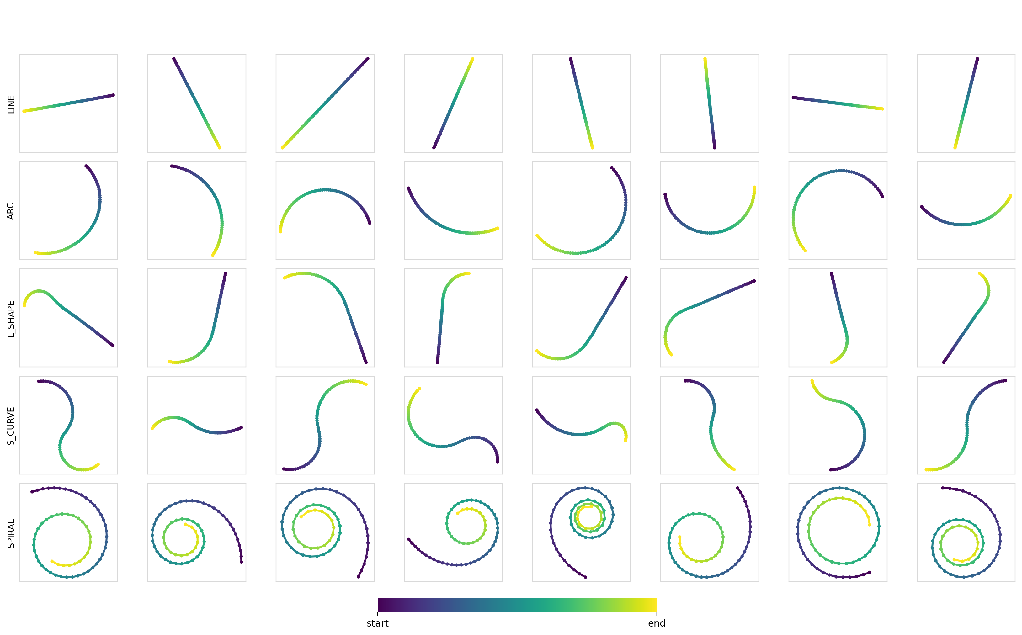
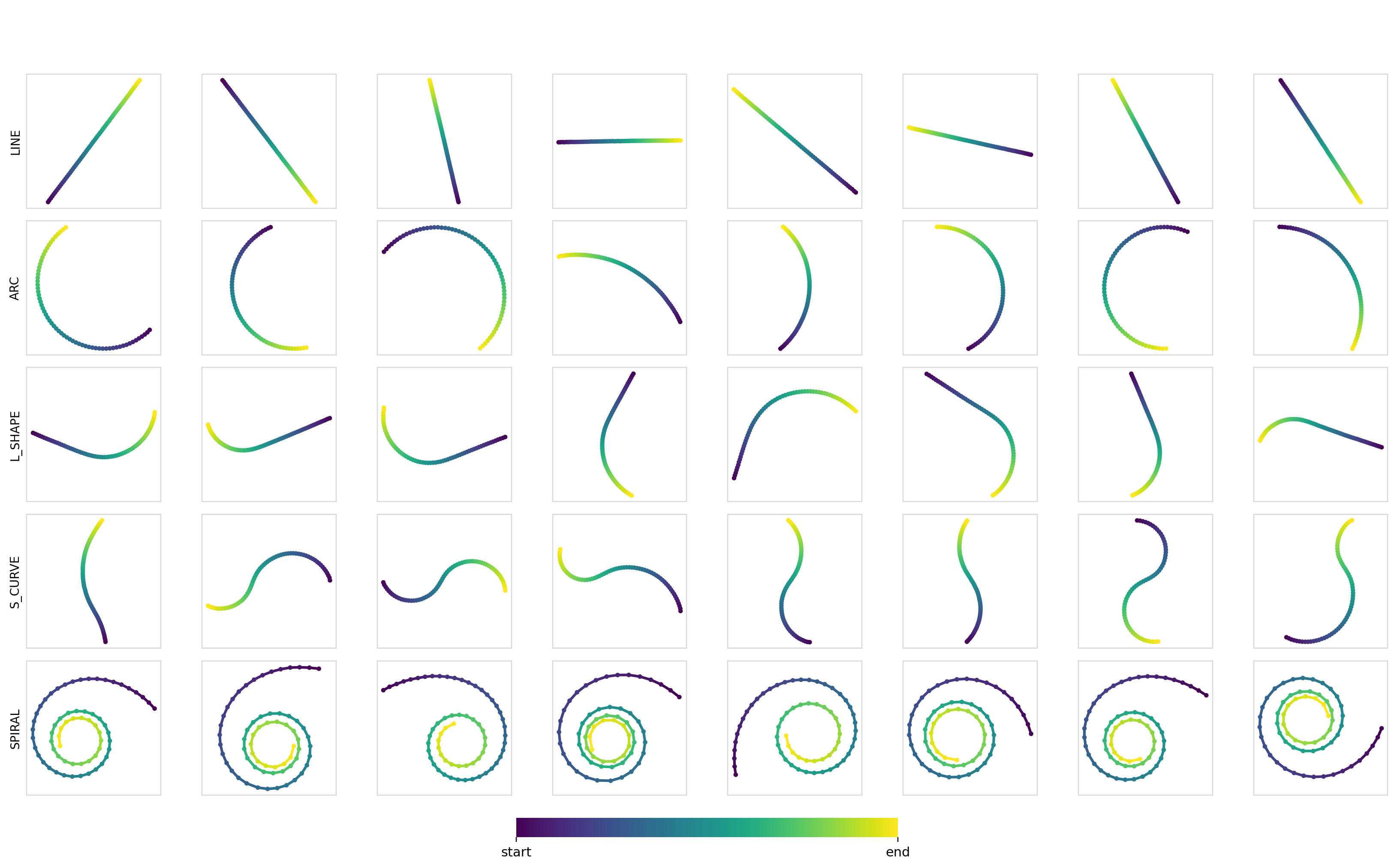
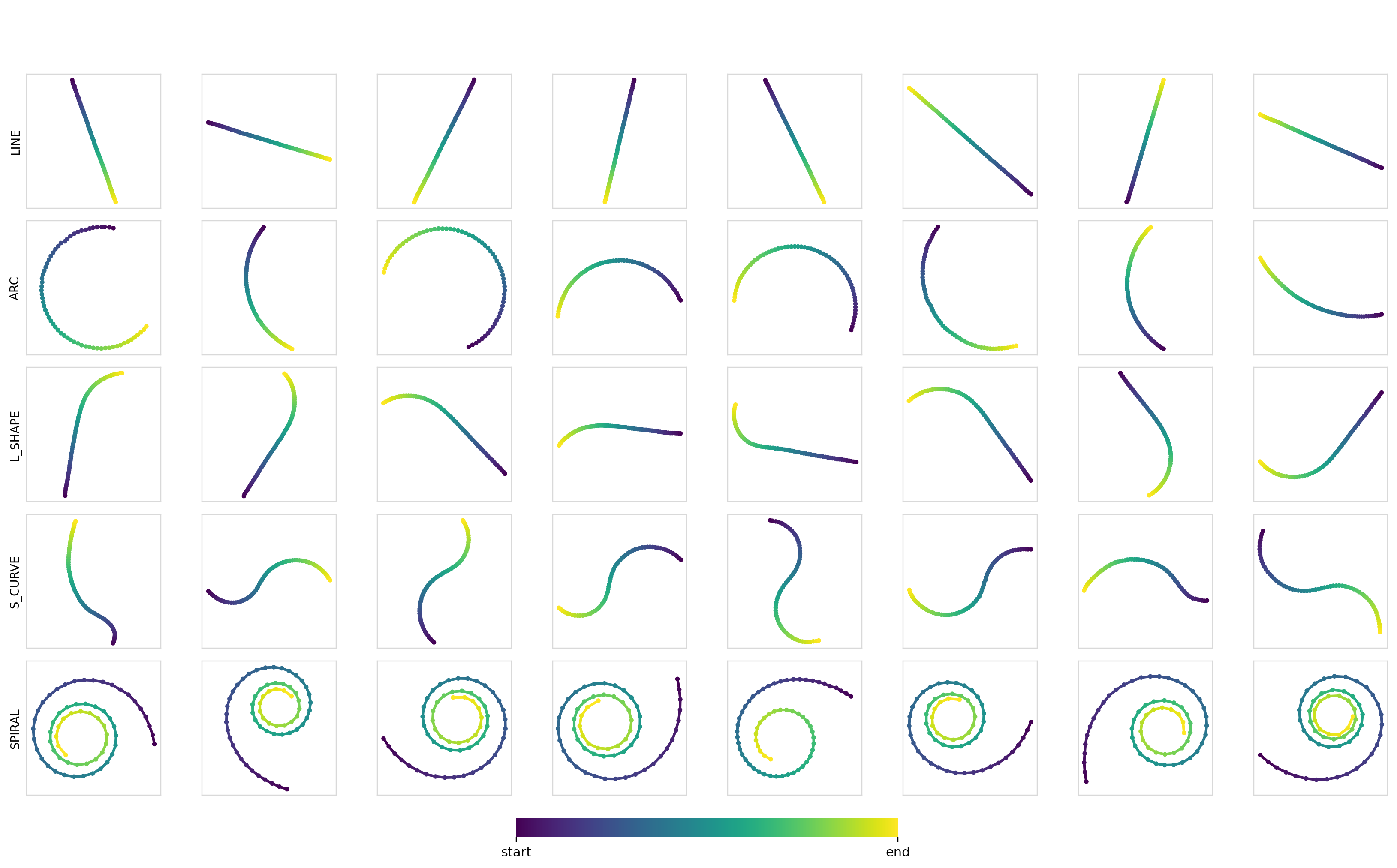
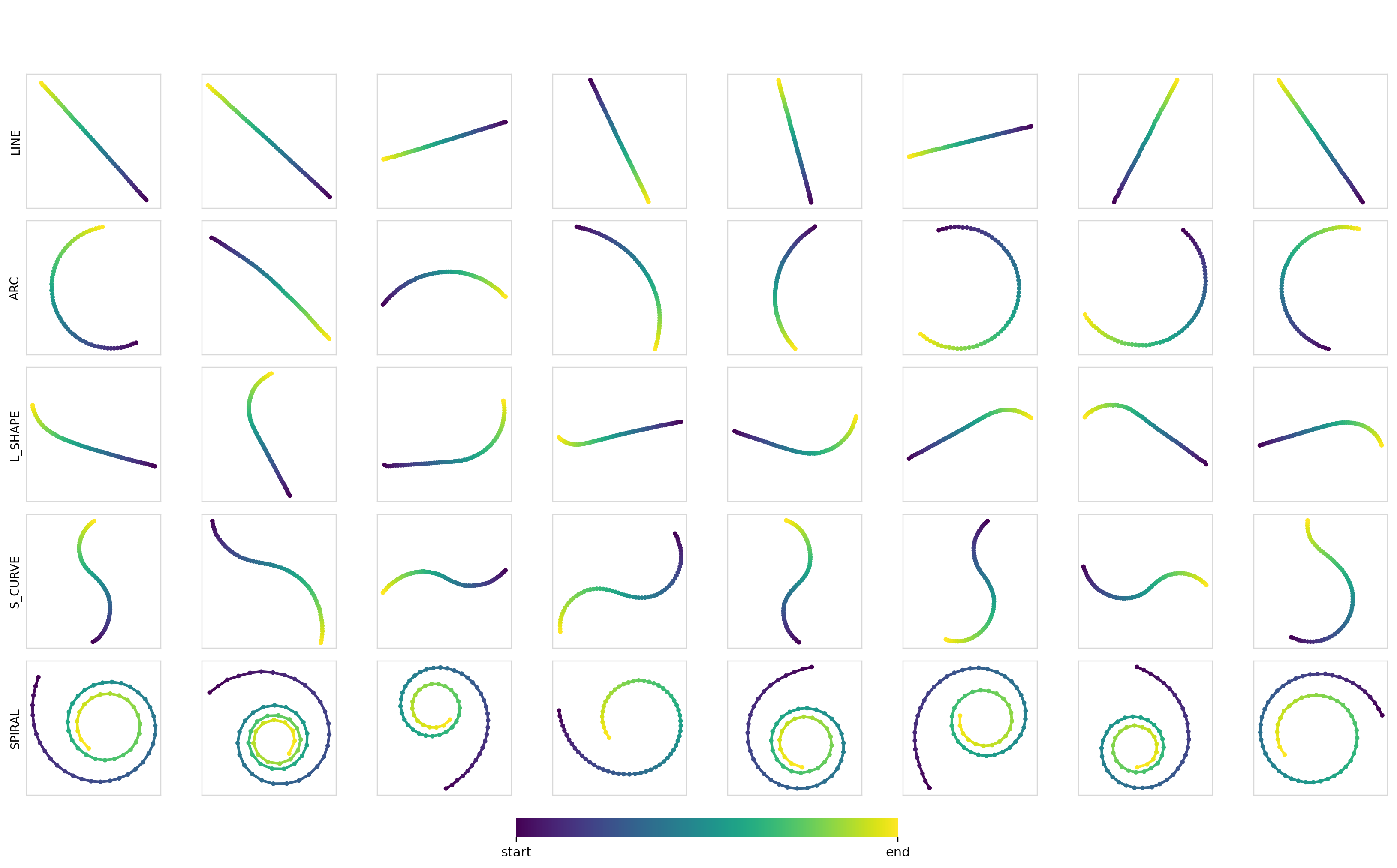
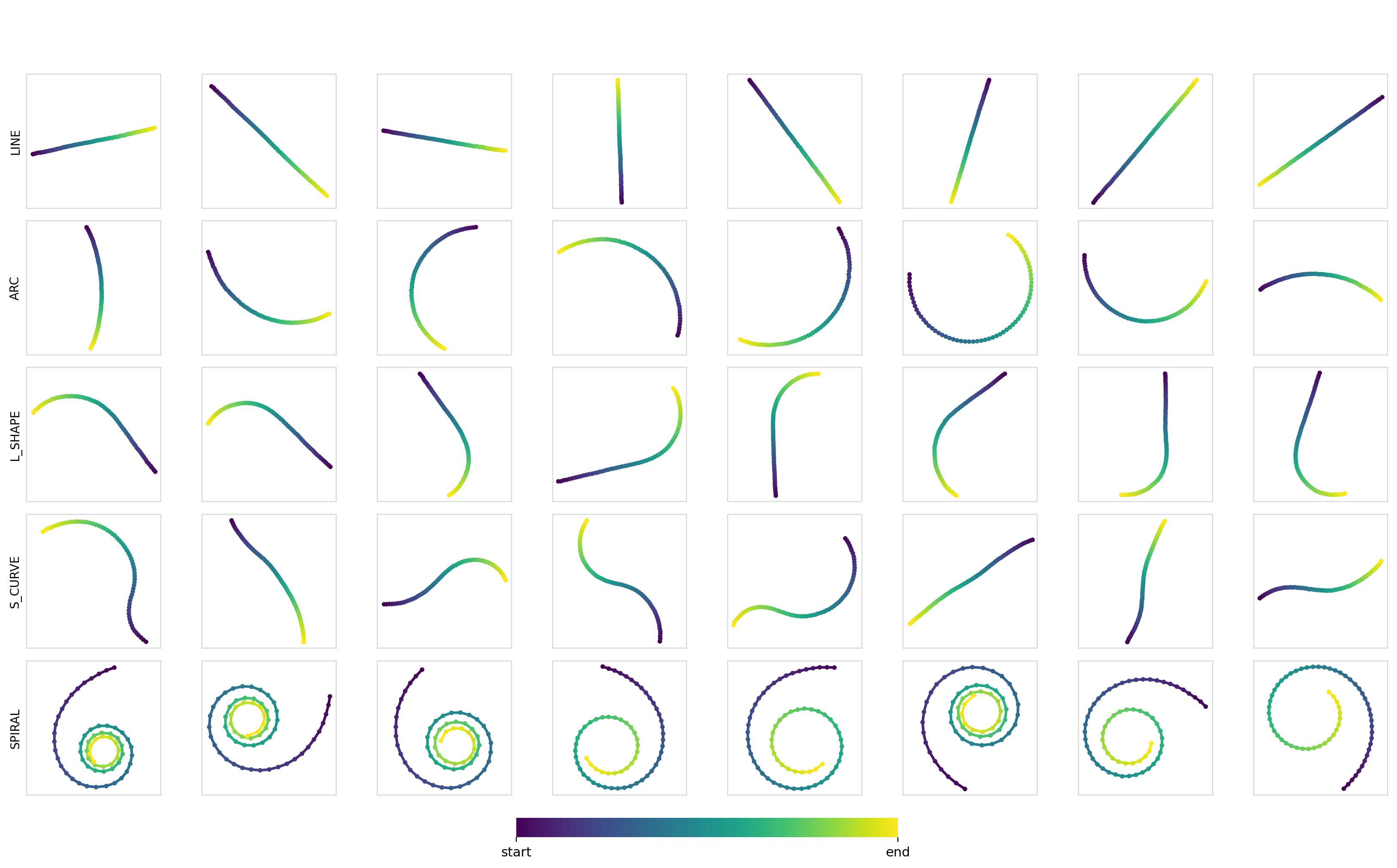
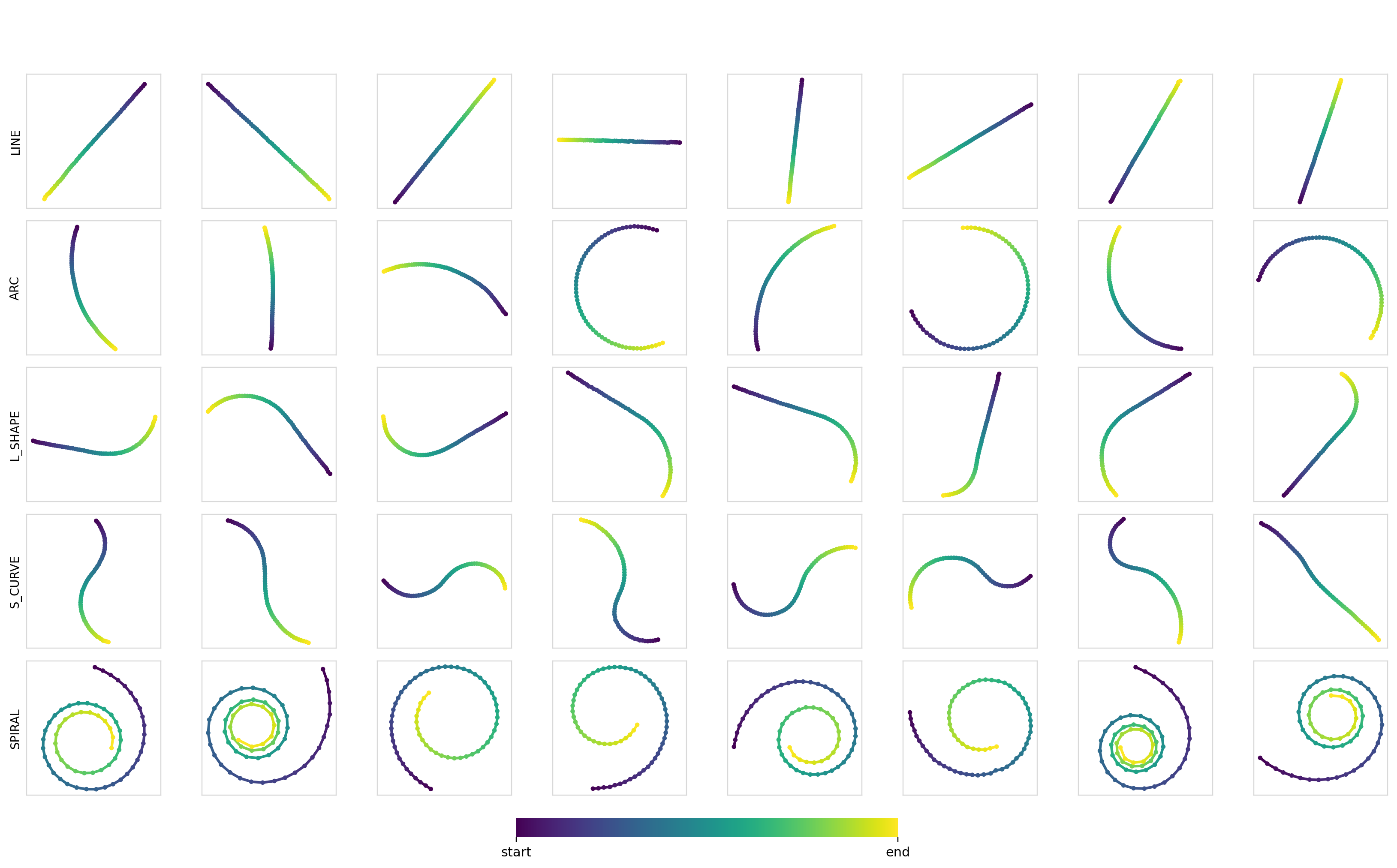
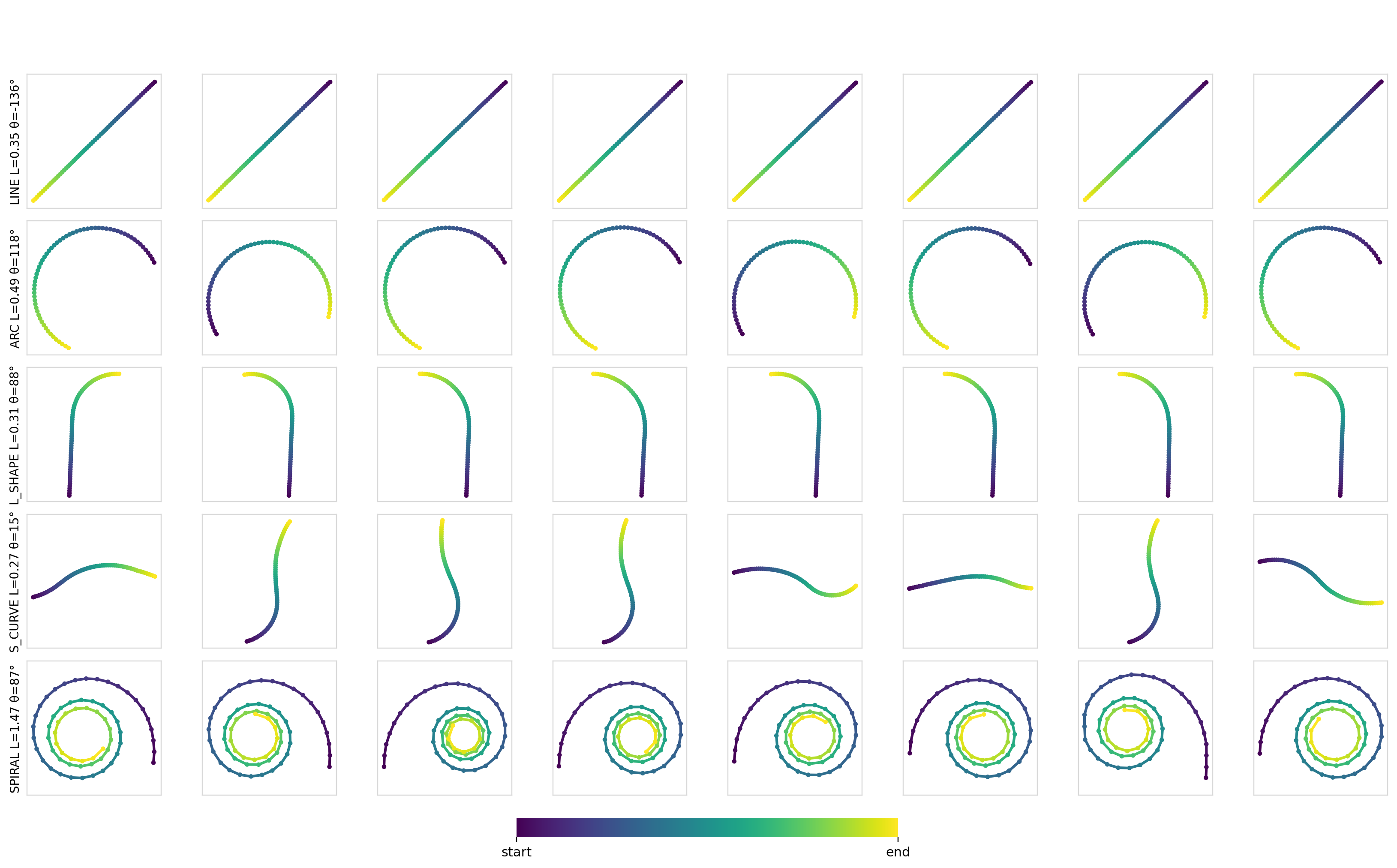
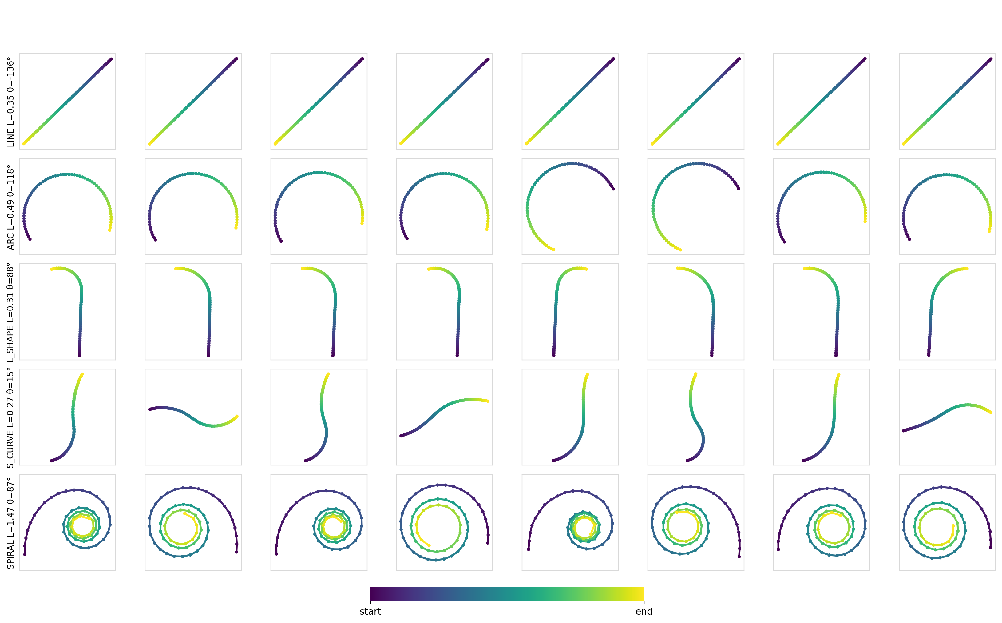
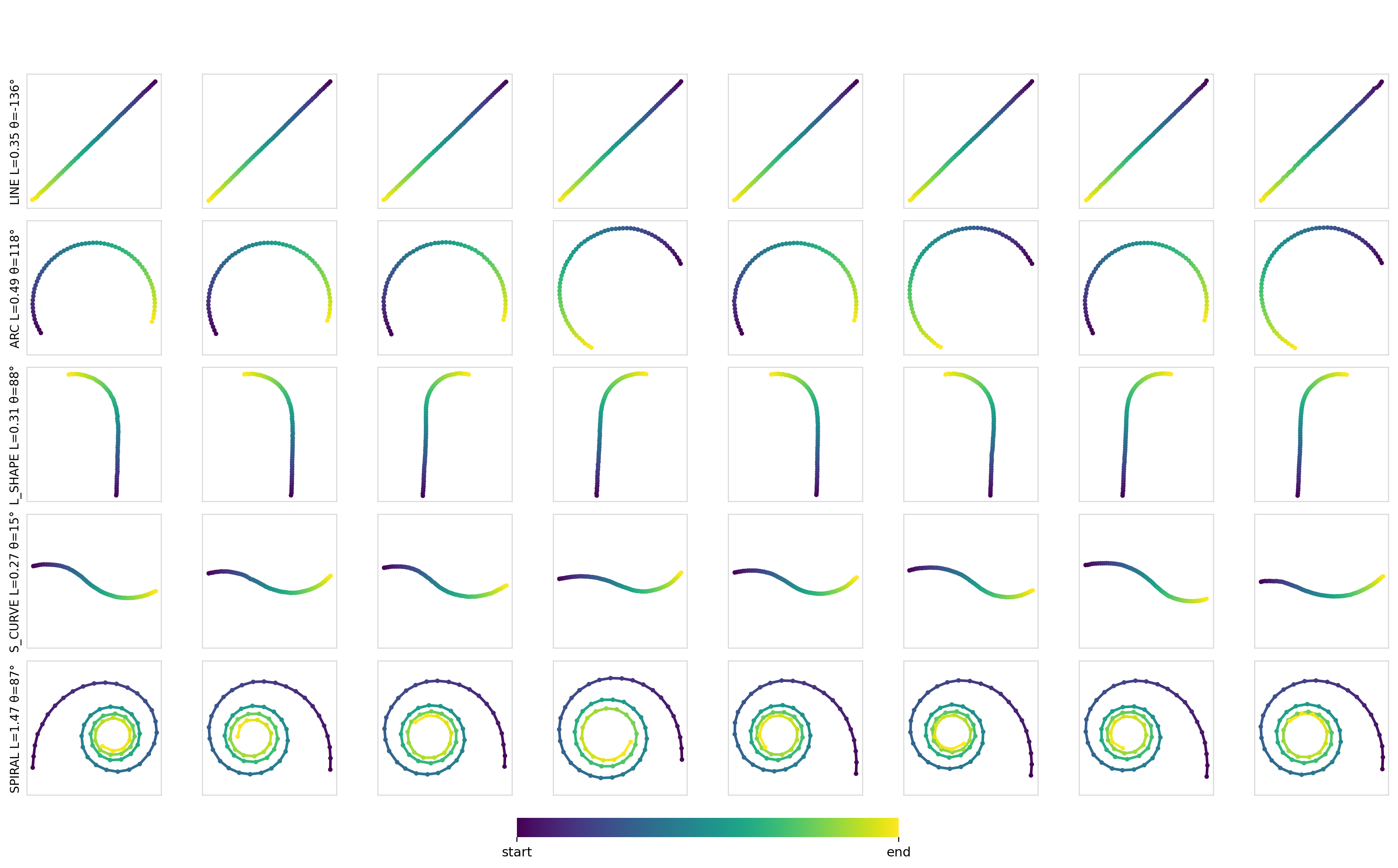
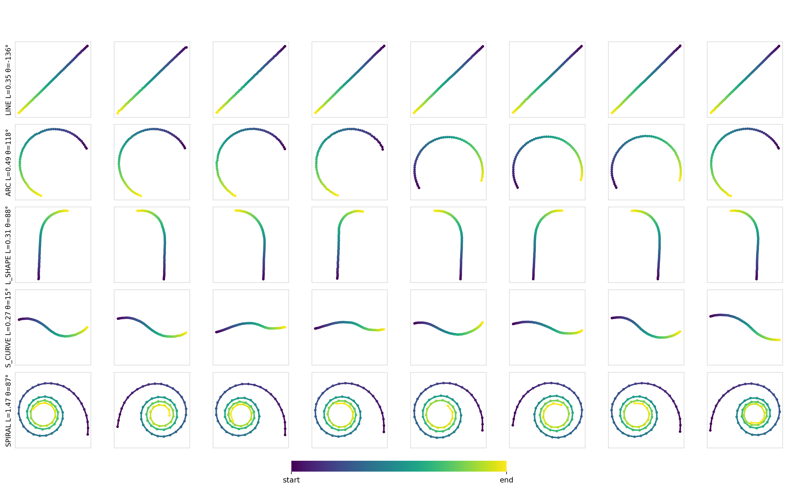
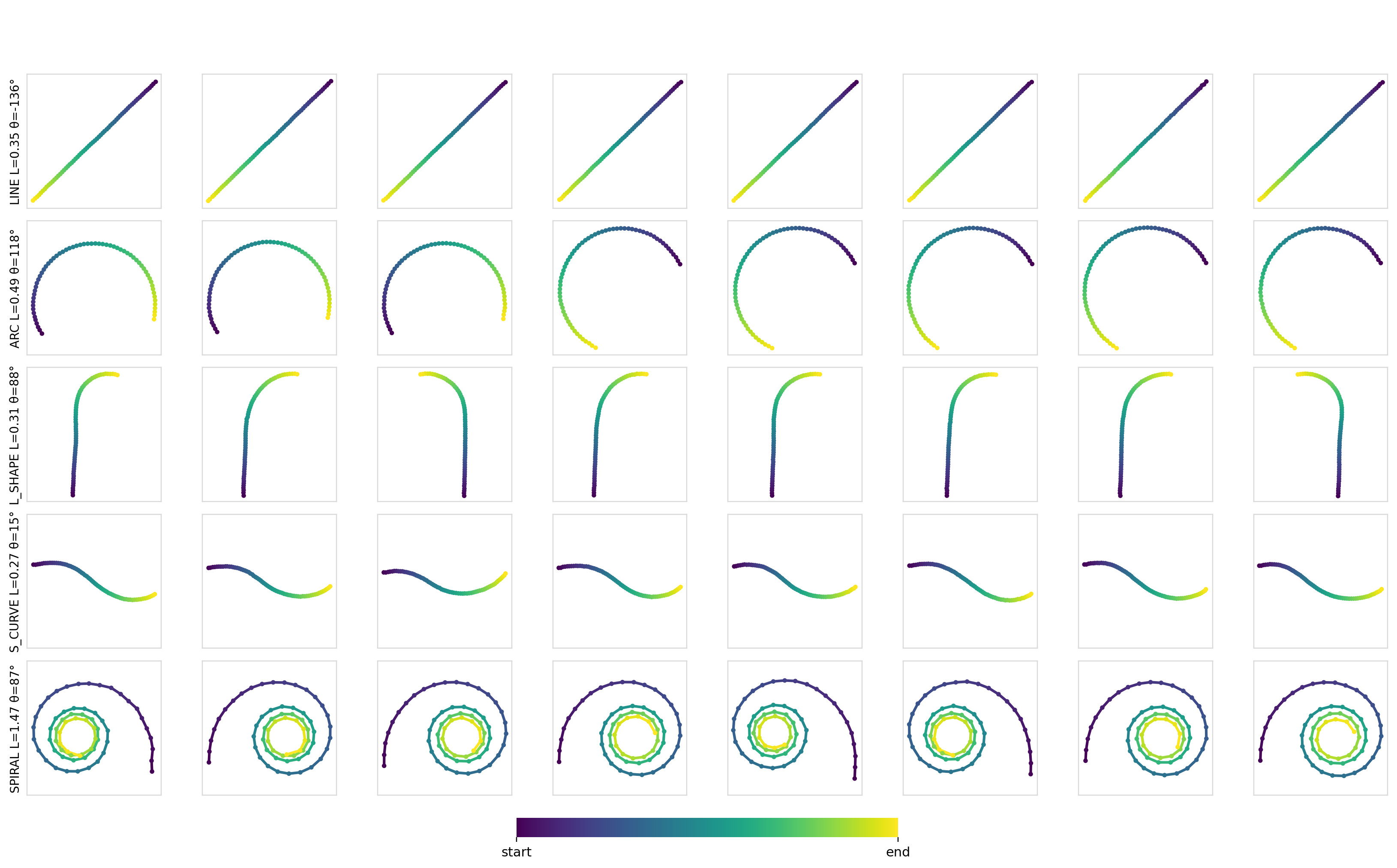
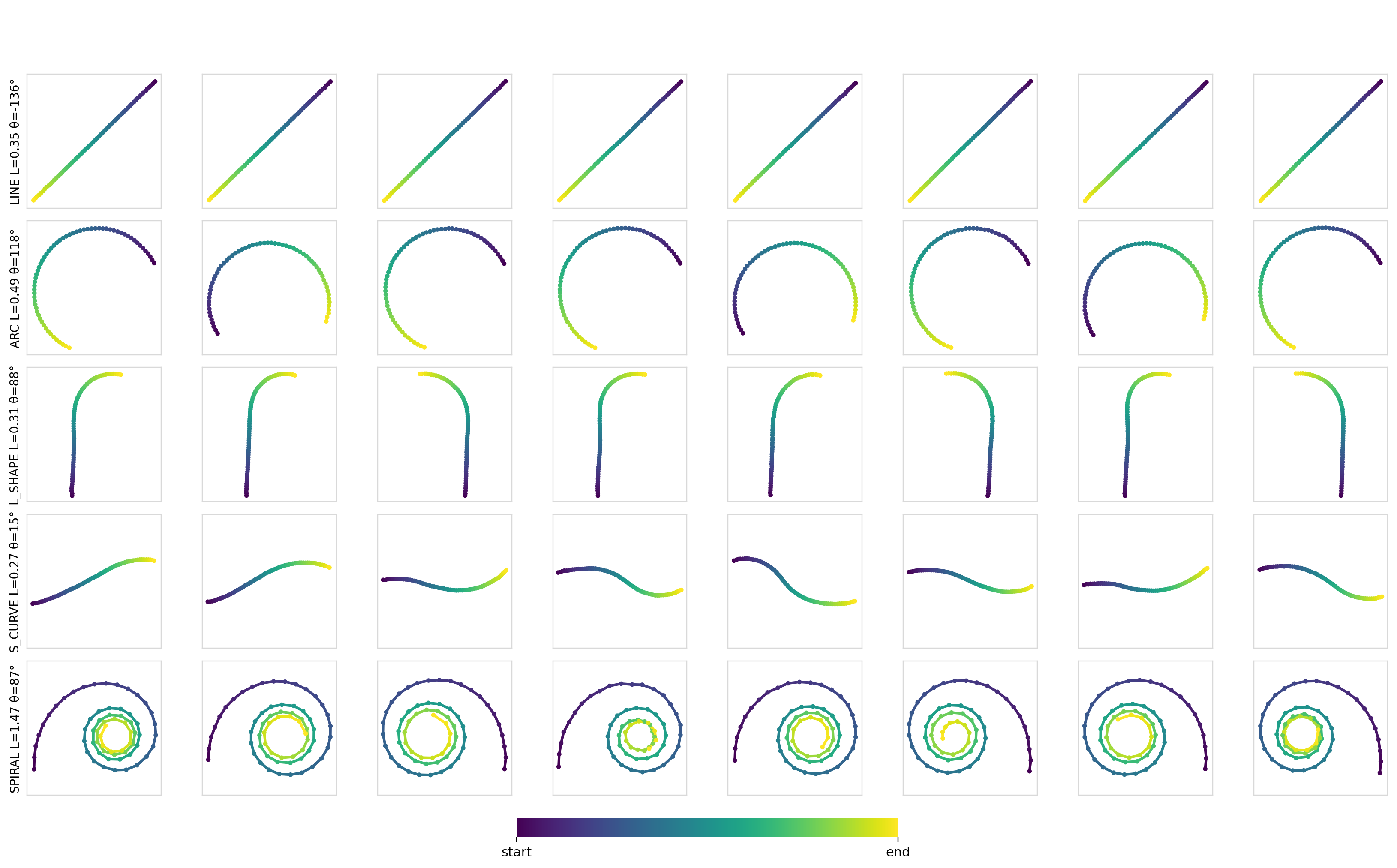
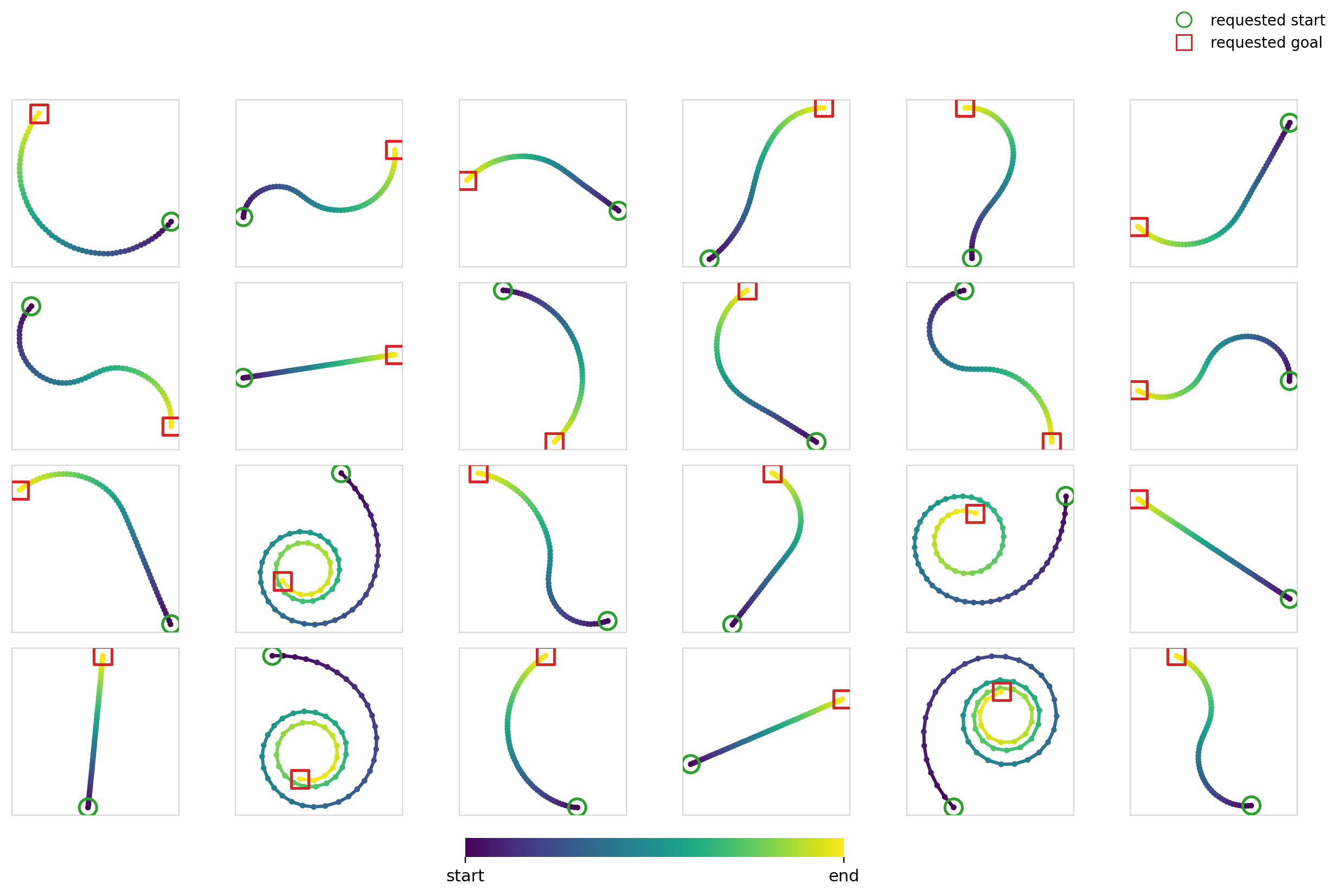
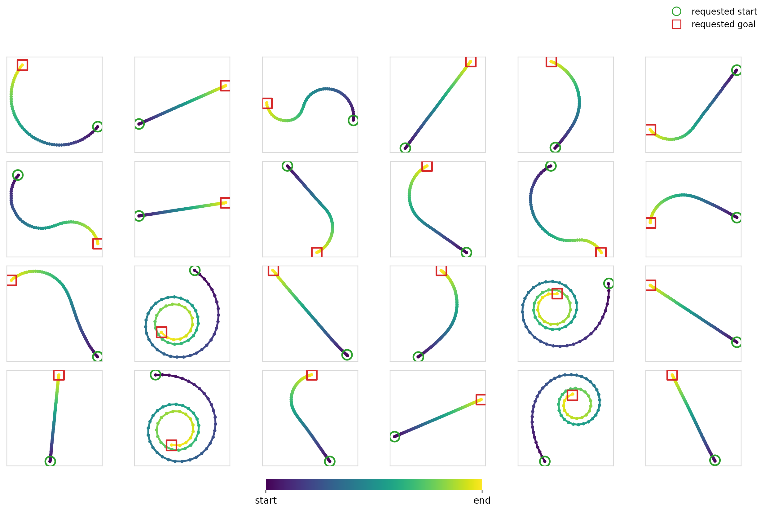
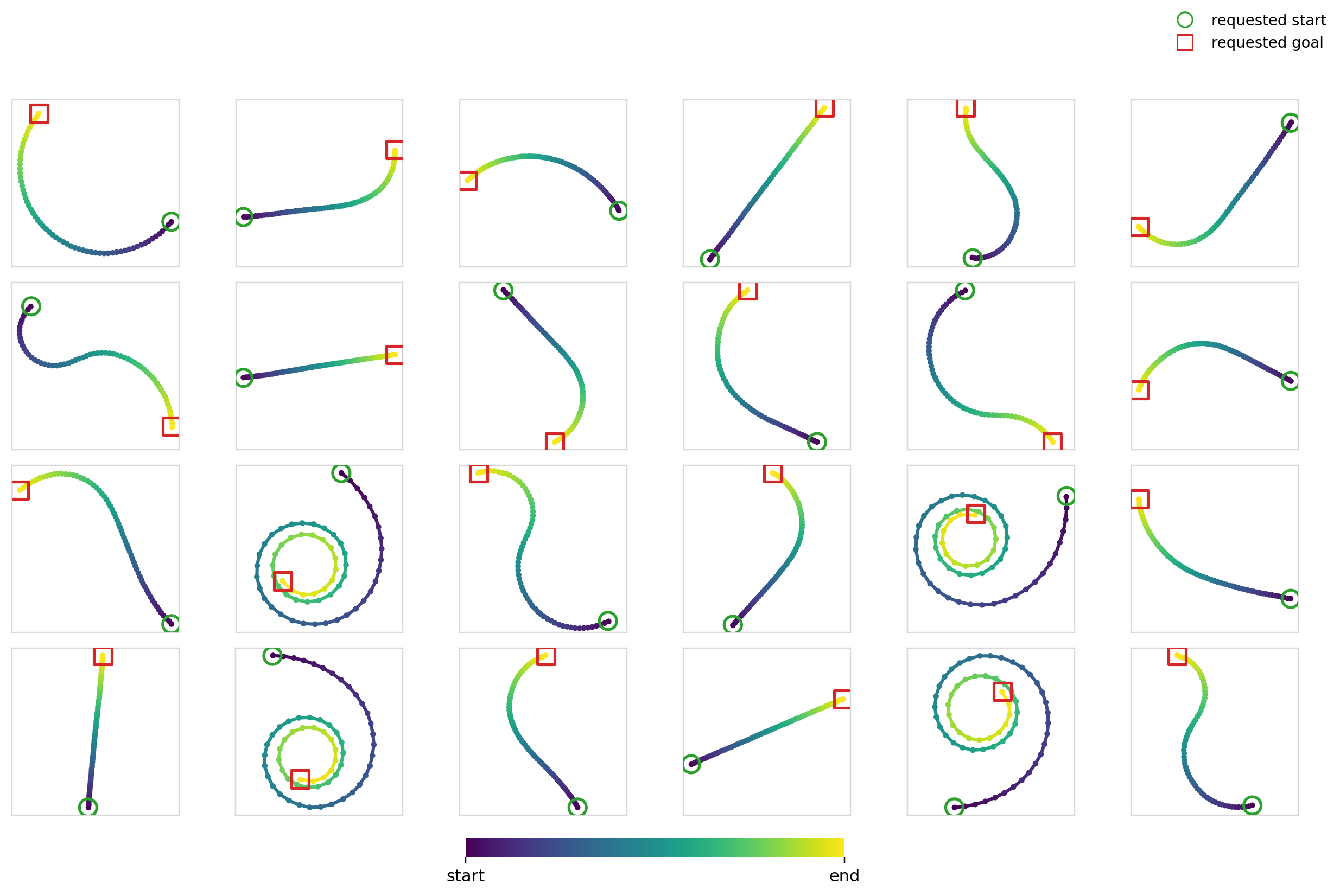
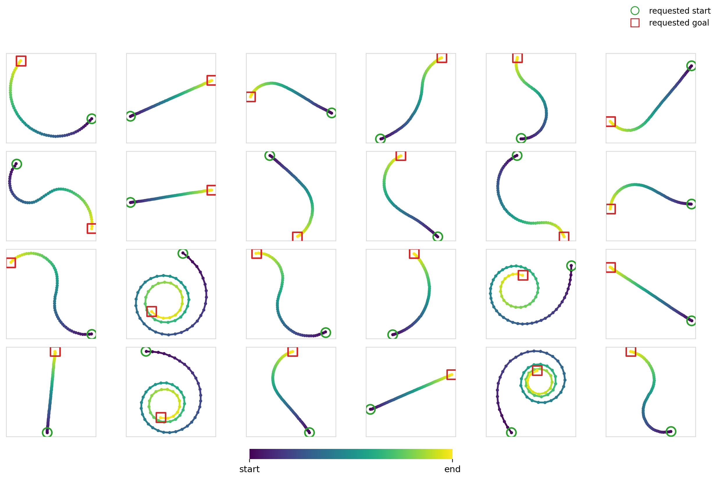
I generated two families of synthetic datasets, both of which are collections of T=64 points bounded in 2-D space. The obvious question is how this scales to more realistic scenarios where we end up with a larger space of actions that includes things like angles. Honestly, I don’t know. We could have more complex inter-point feasibility constraints, etc. for actual robot actions and the results here might not carry over. However, I don’t think that the representation problem differs a lot in terms of complexity. Angles can always be represented with , rotations with 6-D representations, and so on. If the model has enough capacity, it should be able to just figure things out. All that to say, I’d be surprised if most things from this 2-D experiment didn’t translate in some form to more practical problems.
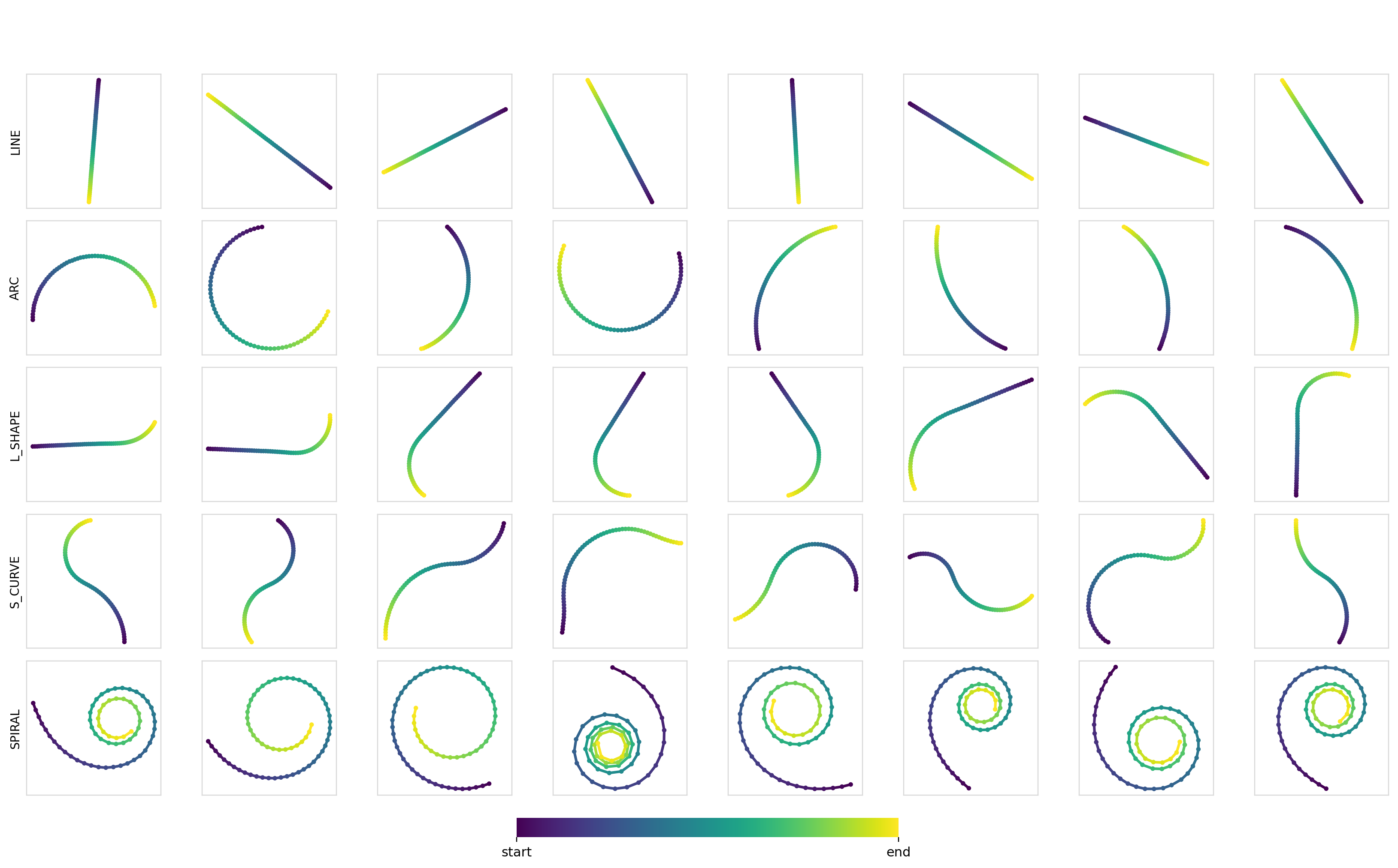
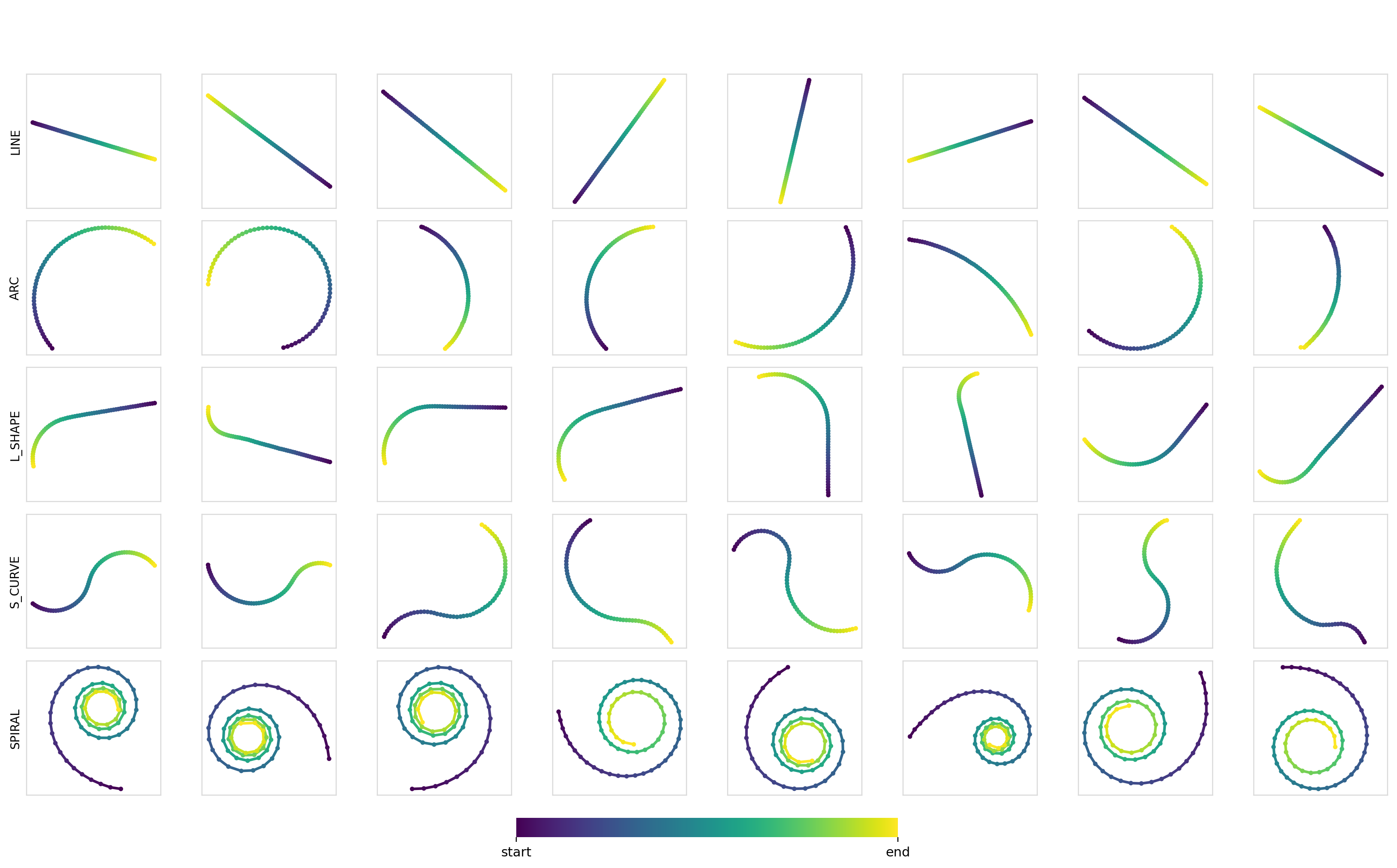
For Dataset1, we sample trajectories from four different classes:
| Class | Fraction | Parameterization | Distribution |
|---|---|---|---|
| Straight line | 0.20 | length , angle | , |
| Constant curvature (Dubins path) | 0.20 | radius , sweep , sign | , , |
| L-shaped | 0.20 | line + Dubins arc | Line and Dubins arc distributions |
| S-shaped | 0.20 | two Dubins arcs, opposite signs | Dubins arc distribution |
| Spiral (Clothoid) | 0.20 | length , start curvature , curvature rate | , , |
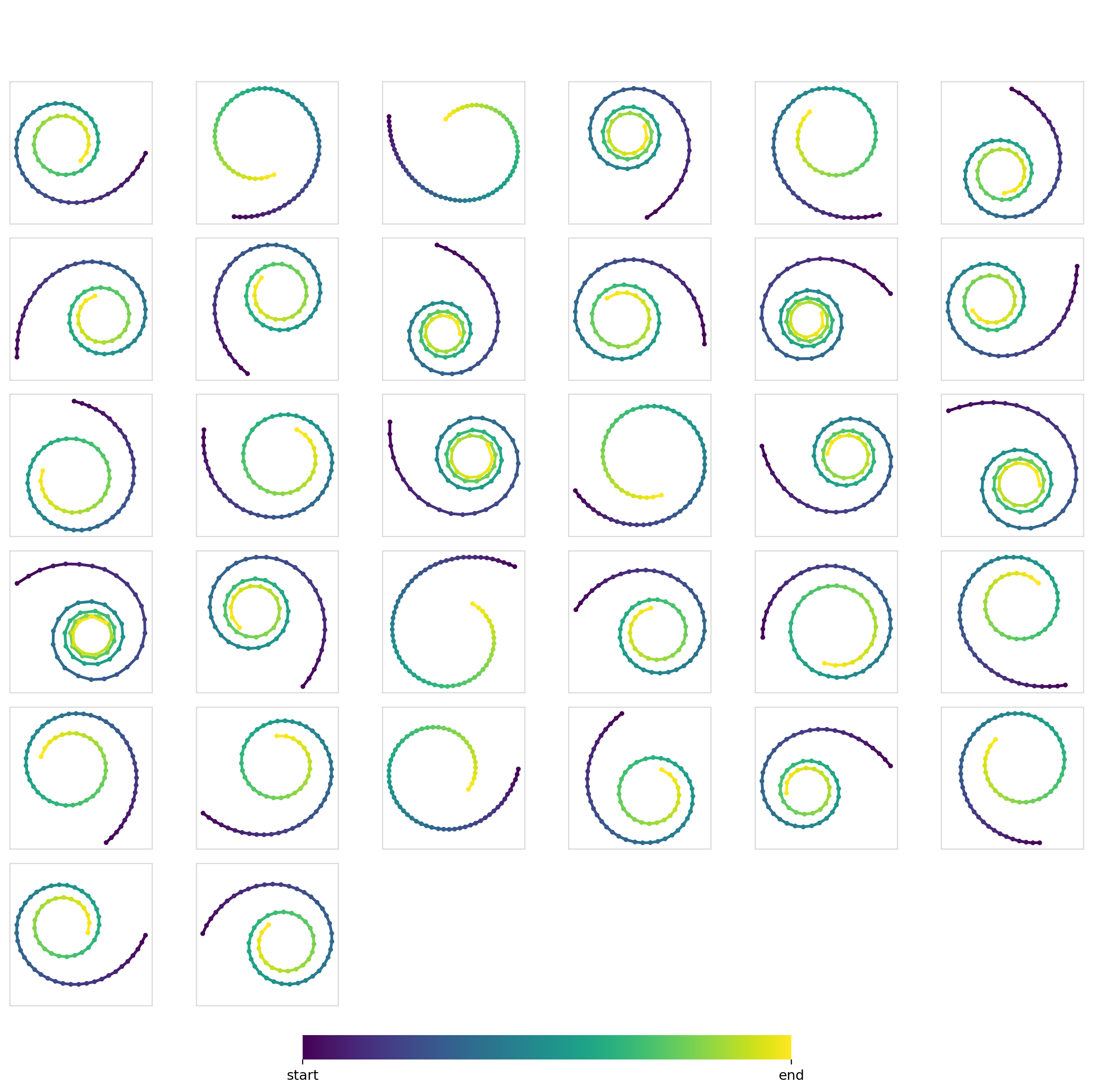
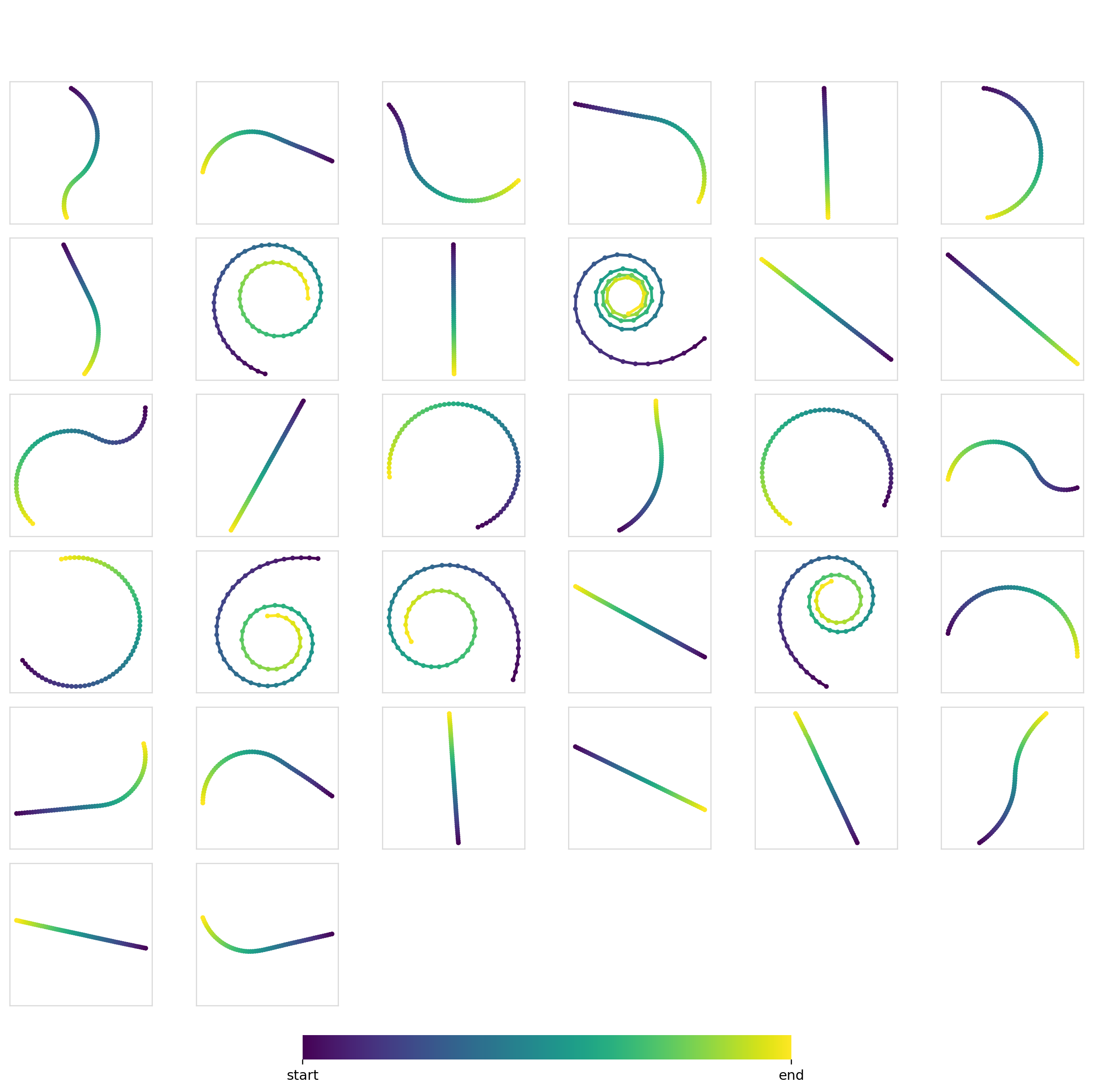
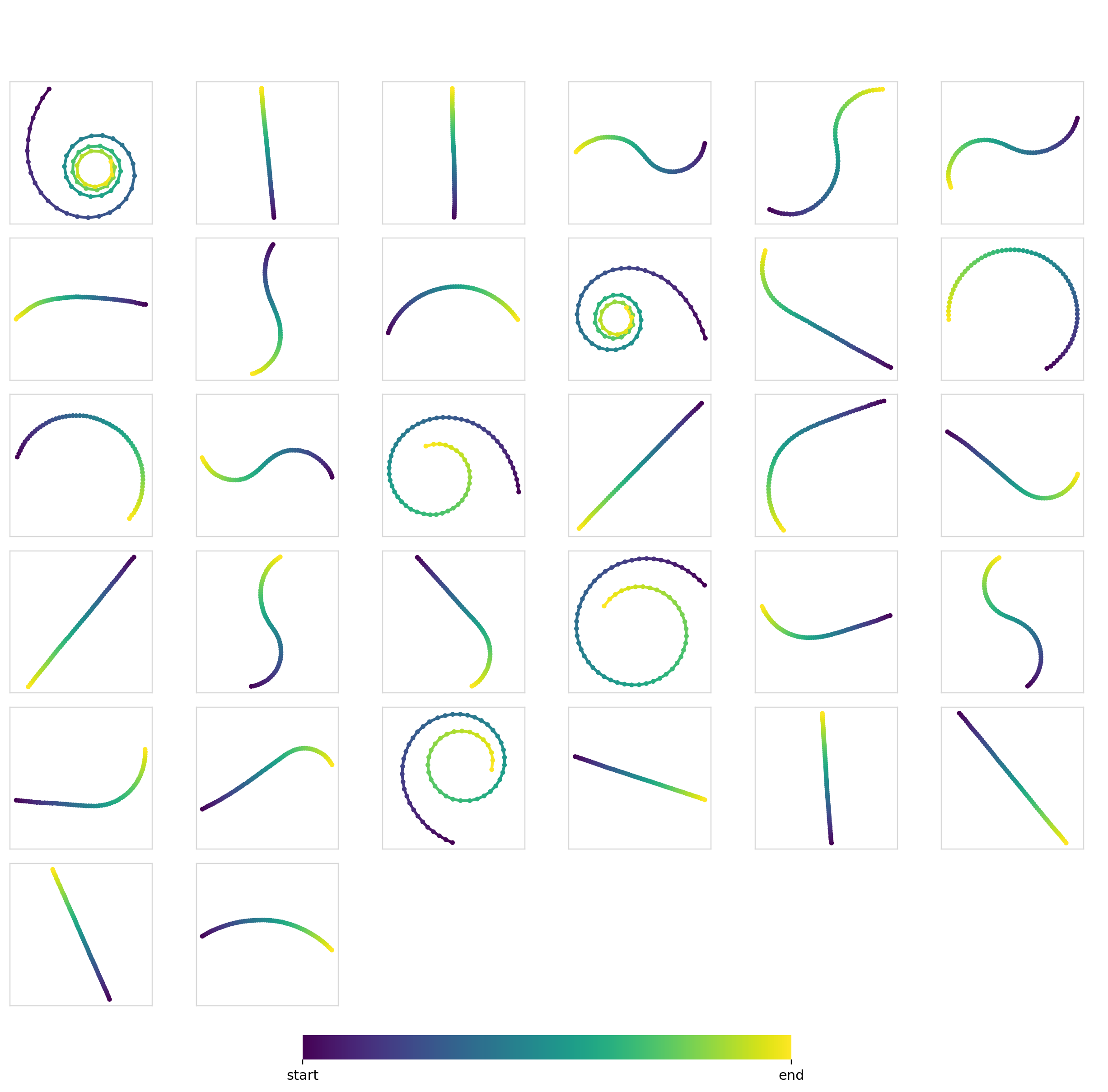
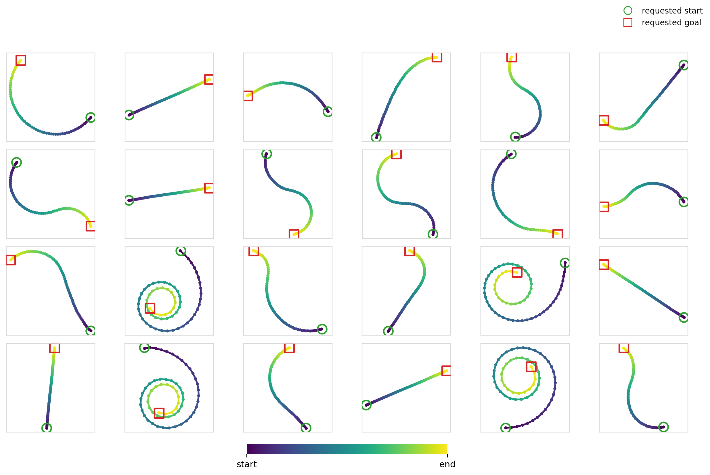
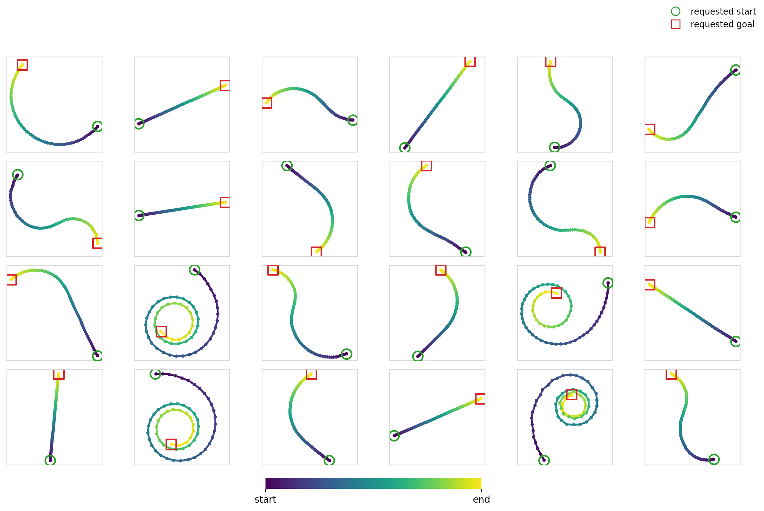
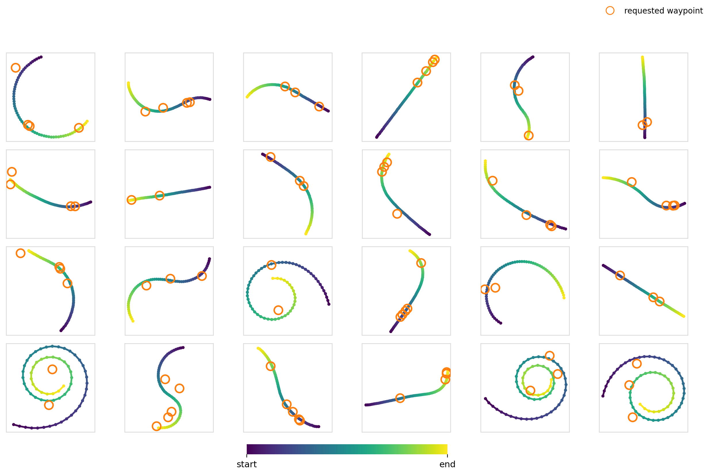
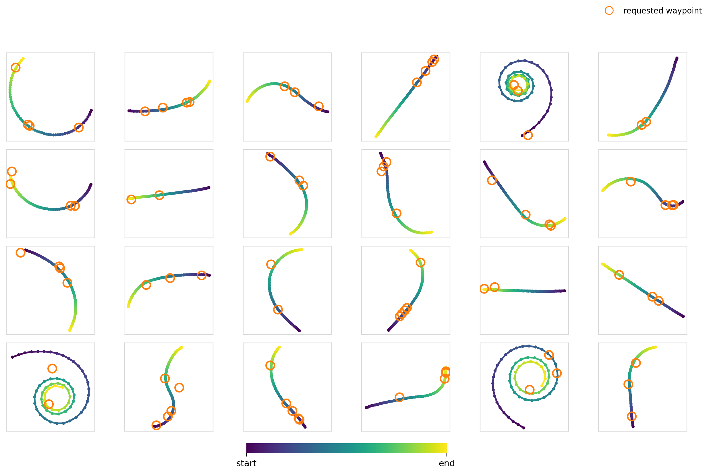
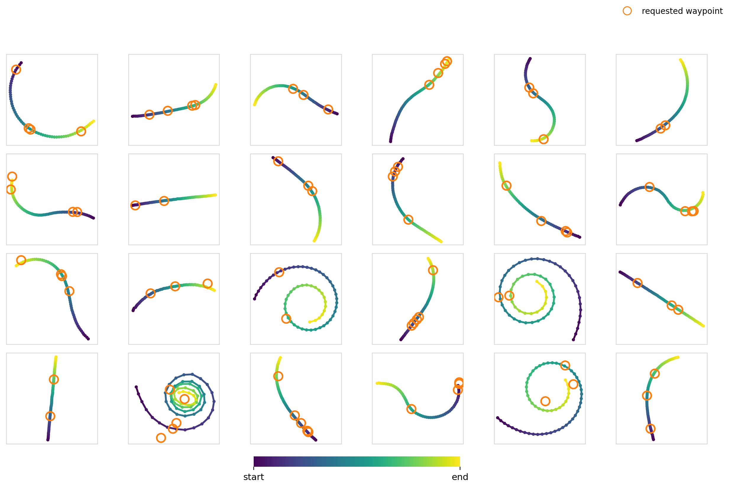
The dataset contains 500,000 trajectories, sampled according to the distributions above. Note that some of the boundaries between the classes are intentionally blurry (Eg: L-shaped and S-shaped trajectories can look quite similar, etc.) to ensure that some of the trivial conditional tasks aren’t too easy. Here’s a gallery of some randomly sampled trajectories:
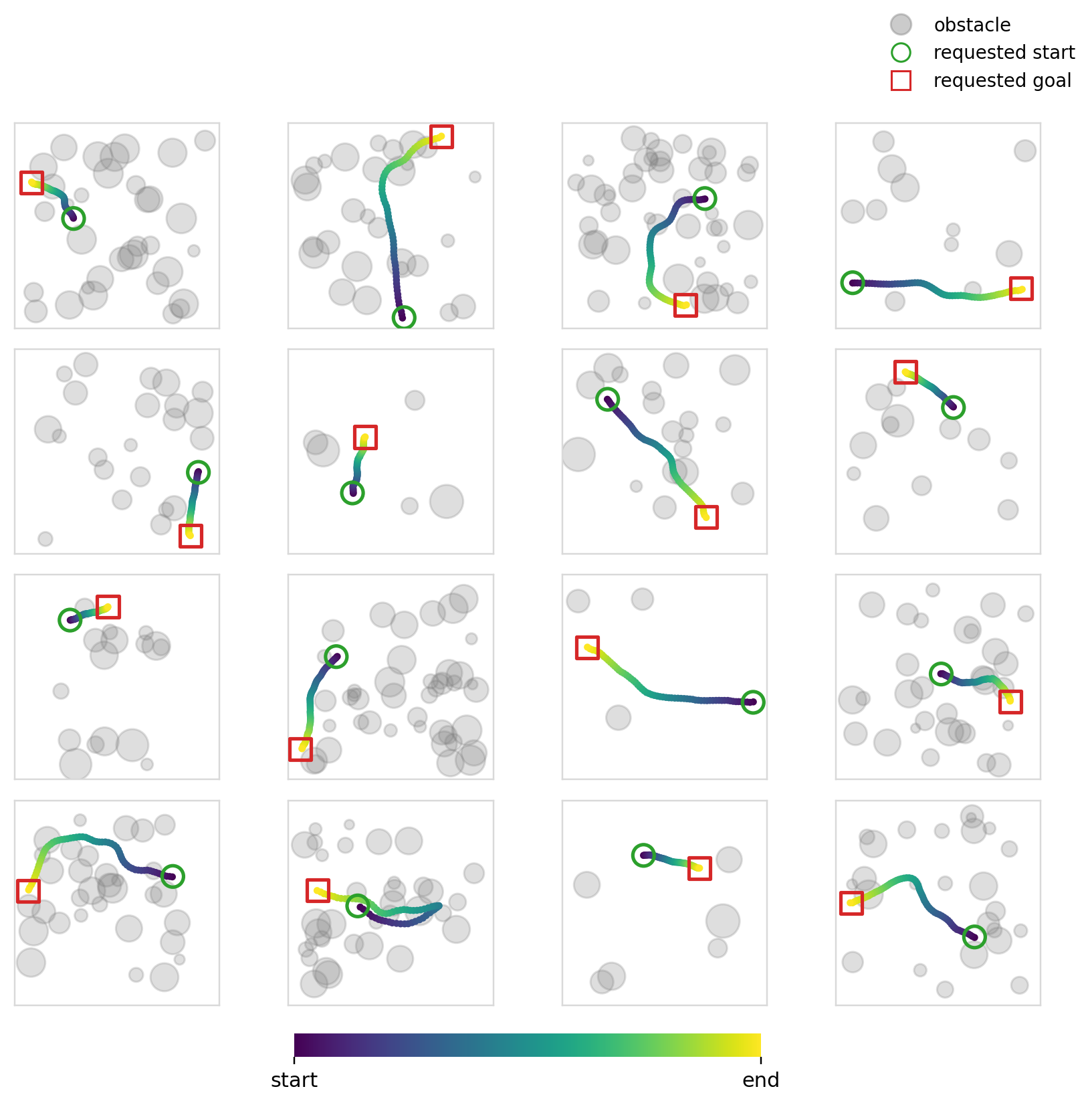
For Dataset2, we generate trajectories in an occupancy map to simulate 2-D path planning. The map is a 64x64 occupancy grid with circular obstacles sampled in the following way:
| Tier | Fraction | Obstacle count | Obstacle radius |
|---|---|---|---|
| Sparse | 0.20 | ||
| Medium | 0.35 | ||
| Dense | 0.45 |
This dataset contains 200,000 trajectories computed by sampling random start and end positions and computing the shortest path between them using A*.
Generative Policies
For the policies, we use a 1-D U-Net structure (as seen in the original Diffusion Policy 4). Each model and conditioning variant uses FiLM for conditioning the timestep (even if the other inputs aren’t conditioned through FiLM). The base model (base U-Net + timestep FiLM) has ~10M parameters.
For diffusion, we train the model to predict the noise . For the samples, we use DDPM 5 (T=100 with a cosine schedule 6). For inference we use DDIM 7 with the 25-50 steps depending on the experiment.
For flow matching 2, we use the same model but predict the velocity instead. During sampling, we sample , and use 10-20 Euler steps during inference. Note that the distribution for is similar to what is used in 8 and is a point of assymetry (compared to diffusion) in our experiments.
Conditioning Methods
FiLM
For FiLM 1, an MLP produces per-channel scale and shift . The inputs get modulated as broadcast over all T actions to produce the (B, C, T) output.
Concat
I wanted to test something that’s a bit more primitive. Concat basically does what it advertises: it concatenates the conditioning feature vector to the input channels (broadcast across T). The (B, C+cond_dim, T) tensor is then projected into (B, C, T).
AdaGN
This one is supposed to be the dressed up version of FiLM. AdaLN-Zero has become popular in DiT networks 9, but given that we’re using 1-D convolutions here, we stick to the group norm. The output is 10, with it starting zero initialized similar to AdaLN-Zero.
Cross-Attention
The only method that applies per timestep conditioning. Queries come from the action trajectory (one per T) with the keys/values coming from the condition tokens. We use multi-head attention with 4 heads 3, with FFN expansions stacked on top for some of the experiments. For single scalar/vector conditioning, this collapses into a single token attention module.
Experiments
Each section here will start with tables outlining the training hyperparameters and model sizes used in the experiment.
Sanity Check
| Policy | Steps | Batch | LR | NFE |
|---|---|---|---|---|
| Diffusion | 20k/80k | 256 | 1e-4 | 25 |
| Flow Matching | 20k/80k | 256 | 1e-4 | 10 |
| FiLM | AdaGN | Concat | Cross-attn |
|---|---|---|---|
| 9.844 | 9.844 | 9.844 | 9.844 |
The first thing to do is to make sure that our base unconditional models work as expected. Training the models on just the spiral trajectories from Dataset1 gives the following output samples:
And no, I couldn’t resist making the classic denoising gif.
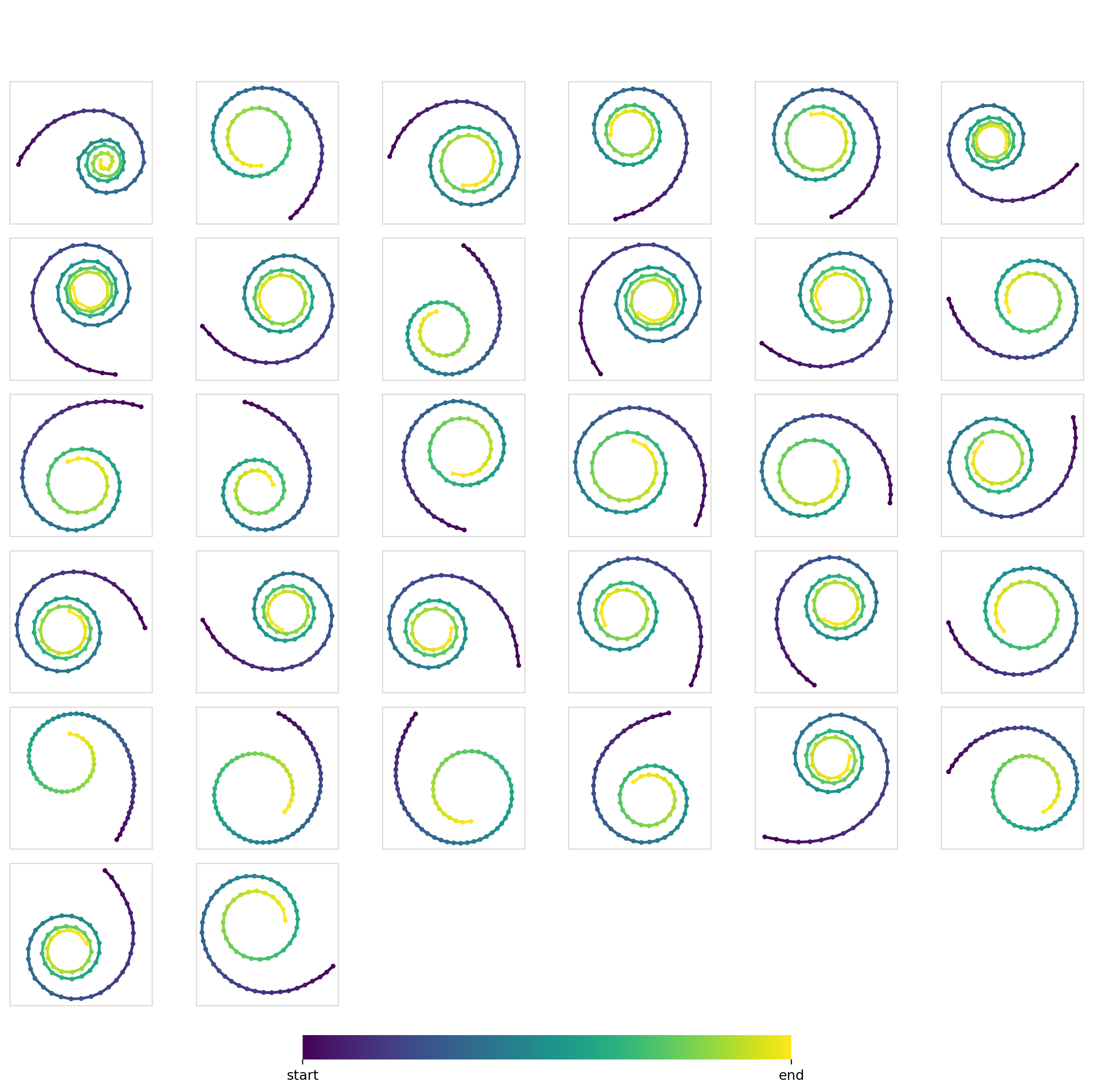
Training unconditionally on all of Dataset1 gives you samples from every class as expected.
Experiment 1
| Policy | Steps | Batch | LR | NFE |
|---|---|---|---|---|
| Diffusion | 40k | 256 | 1e-4 | 25 |
| Flow Matching | 40k | 256 | 1e-4 | 10 |
| FiLM | AdaGN | Concat | Cross-attn |
|---|---|---|---|
| 9.872 | 9.872 | 8.918 | 10.167 |
We start with something very simple: conditioning on the trajectory class (in Dataset1). The class input is encoded as a one-hot vector (dim=5).
We want to ensure two things:
- The models are able to produce trajectories of the given class
- The models exhibit diversity within trajectories of the same class
The first thing here isn’t trivial to verify. To do this we train a small 1-D convolution classifier. The classifier has an ~100% accuracy on a generated validation dataset, so we can go ahead and use it to gauge the accuracy of conditioning.
| Diffusion | Flow Matching | |
|---|---|---|
| FiLM | 0.988 | 0.985 |
| AdaGN | 0.995 | 0.980 |
| Concat | 0.991 | 0.986 |
| Cross-attn | 0.987 | 0.993 |
The accuracies aren’t 1.0 but given that the boundaries between the classes aren’t that distinct, we’ll give the models a pass. Unsurprisingly, we don’t see any differences between the conditioning mechanisms or the models for this task.
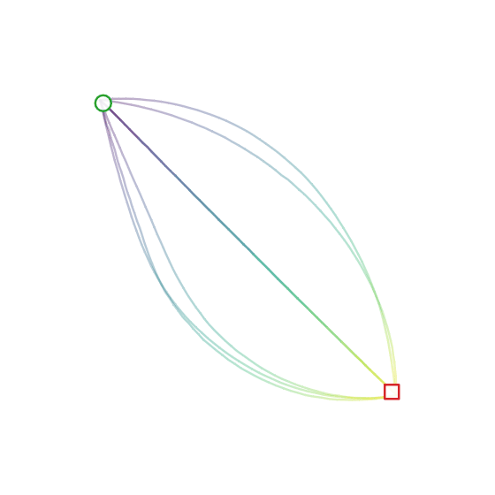
We can also measure the diversity (pairwise Euclidean distance between trajectories) of the samples within each class. These turn out to be pretty good at ~7.5-8.0, with the values being smaller for the line trajectories and larger for curves and arcs. Samples for each combination:
Experiment 2
| Policy | Steps | Batch | LR | NFE |
|---|---|---|---|---|
| Diffusion | 40k | 256 | 1e-4 | 25 |
| Flow Matching | 40k | 256 | 1e-4 | 10 |
| FiLM | AdaGN | Concat | Cross-attn |
|---|---|---|---|
| 9.890 | 9.890 | 8.927 | 10.184 |
Now we step it up a bit and condition the trajectories on the class, trajectory length and initial heading. The class is still encoded as a one-hot vector, with the length and angles represented as regular floats. To handle angle wrapping, we represent it as (, ). Stacking everything together, we end up with a single dim=8 vector.
We use the same Oracle to measure classification accuracy:
| Diffusion | Flow Matching | |
|---|---|---|
| FiLM | 0.966 | 0.982 |
| AdaGN | 0.973 | 0.972 |
| Concat | 0.966 | 0.980 |
| Cross-attn | 0.963 | 0.968 |
The accuracy spread is all due to the curve classes as expected. The error in length is 0.001-0.017 and the error in the angle is 1-10 deg, with no notable differences between any of the configurations.
Here are some samples for a given set of constraints:
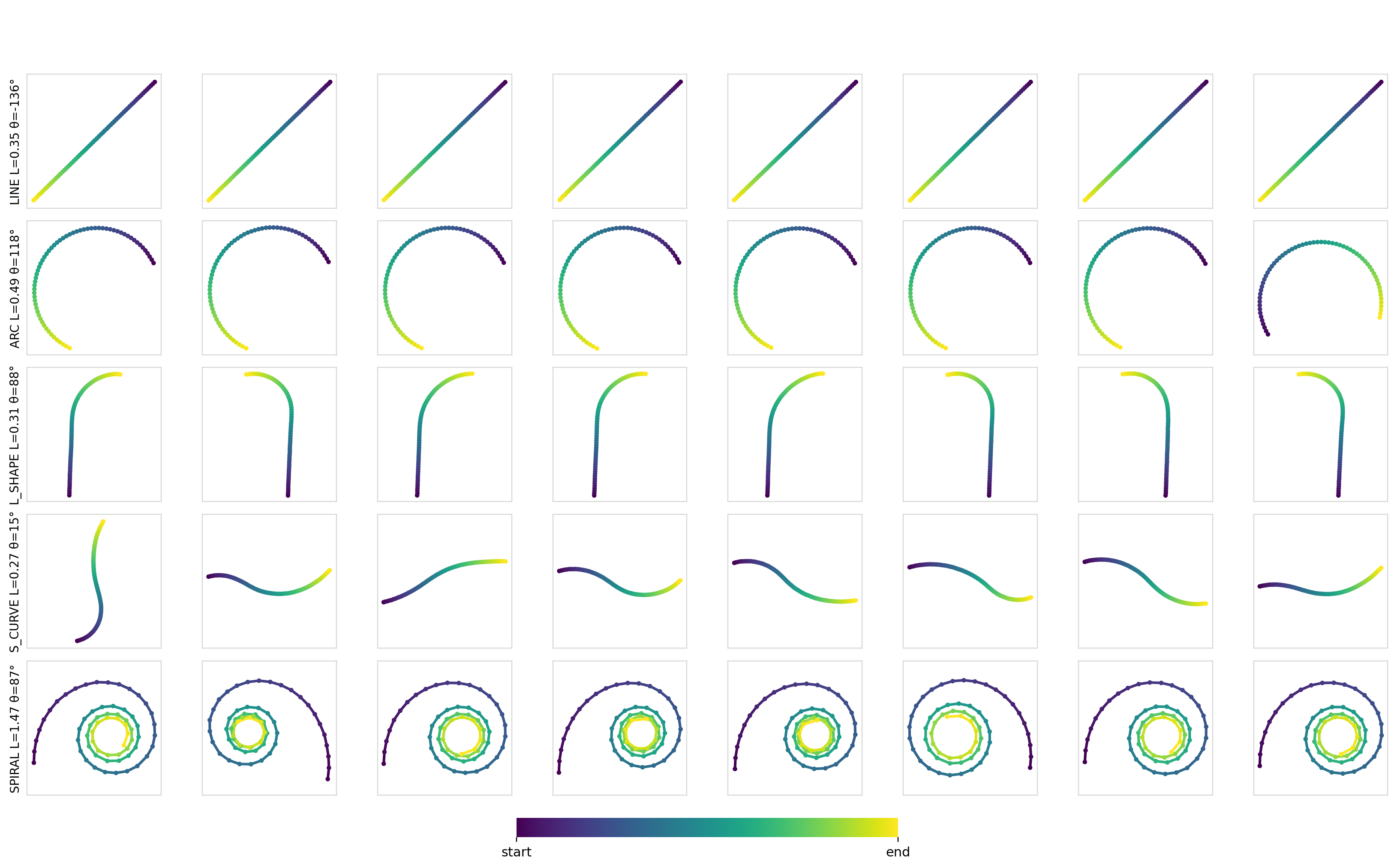
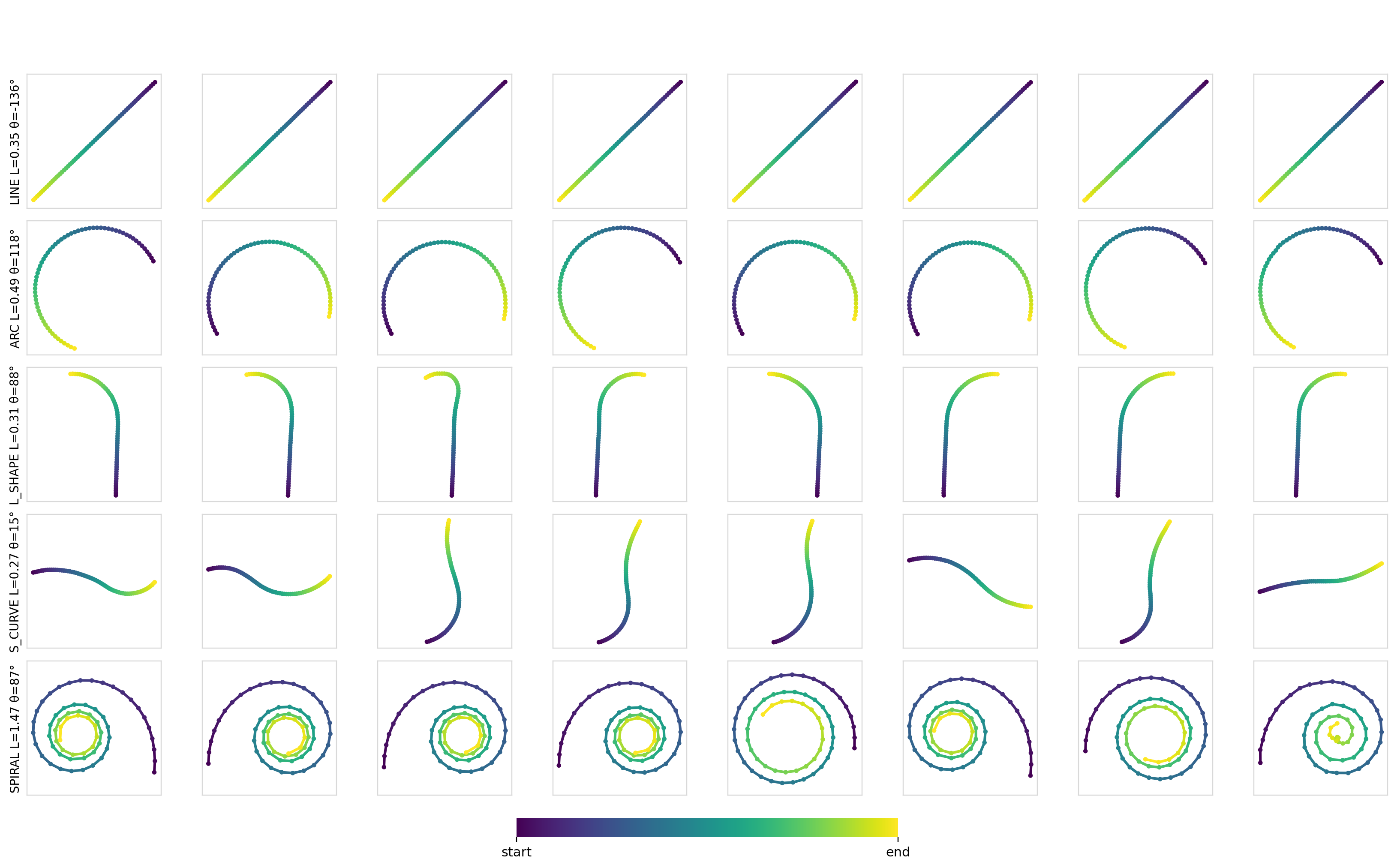
As expected, for simple conditioning, there aren’t any differences between any of the mechanisms or models. Applying conditioning globally across all of the timesteps is more than sufficient to encode such conditioning information and drive the output.
Experiment 3
| Policy | Steps | Batch | LR | NFE |
|---|---|---|---|---|
| Diffusion | 40k | 256 | 1e-4 | 25 |
| Flow Matching | 40k | 256 | 1e-4 | 10 |
| FiLM | AdaGN | Concat | Cross-attn |
|---|---|---|---|
| 9.867 | 9.867 | 8.915 | 10.161 |
We now condition the start and endpoints of the trajectory. We end up with a smaller dim=4 conditioning vector but requires more local structure as the start and endpoints are fixed. I expected the global methods to do slightly worse. They didn’t.
| Diffusion | Flow Matching | |
|---|---|---|
| FiLM | 0.0035 ± 0.0016 | 0.0056 ± 0.0012 |
| AdaGN | 0.0056 ± 0.0022 | 0.0089 ± 0.0033 |
| Concat | 0.0040 ± 0.0022 | 0.0069 ± 0.0024 |
| Cross-attn | 0.0057 ± 0.0026 | 0.0073 ± 0.0027 |
FiLM performed the best consistently, but they’re all very close. Turns out that the spatial constraints are simple enough that pooling them through the entire trajectory (along with some convolution magic) is sufficient to solve the problem. But then again, this makes sense given how U-Nets work.
Here’s the diffusion + FiLM model in action:
Experiment 4
| Policy | Steps | Batch | LR | NFE |
|---|---|---|---|---|
| Diffusion | 40k | 256 | 1e-4 | 50 |
| Flow Matching | 40k | 256 | 1e-4 | 20 |
| FiLM | AdaGN | Concat | Cross-attn |
|---|---|---|---|
| 13.408 | 13.408 | 12.534 | 14.075 |
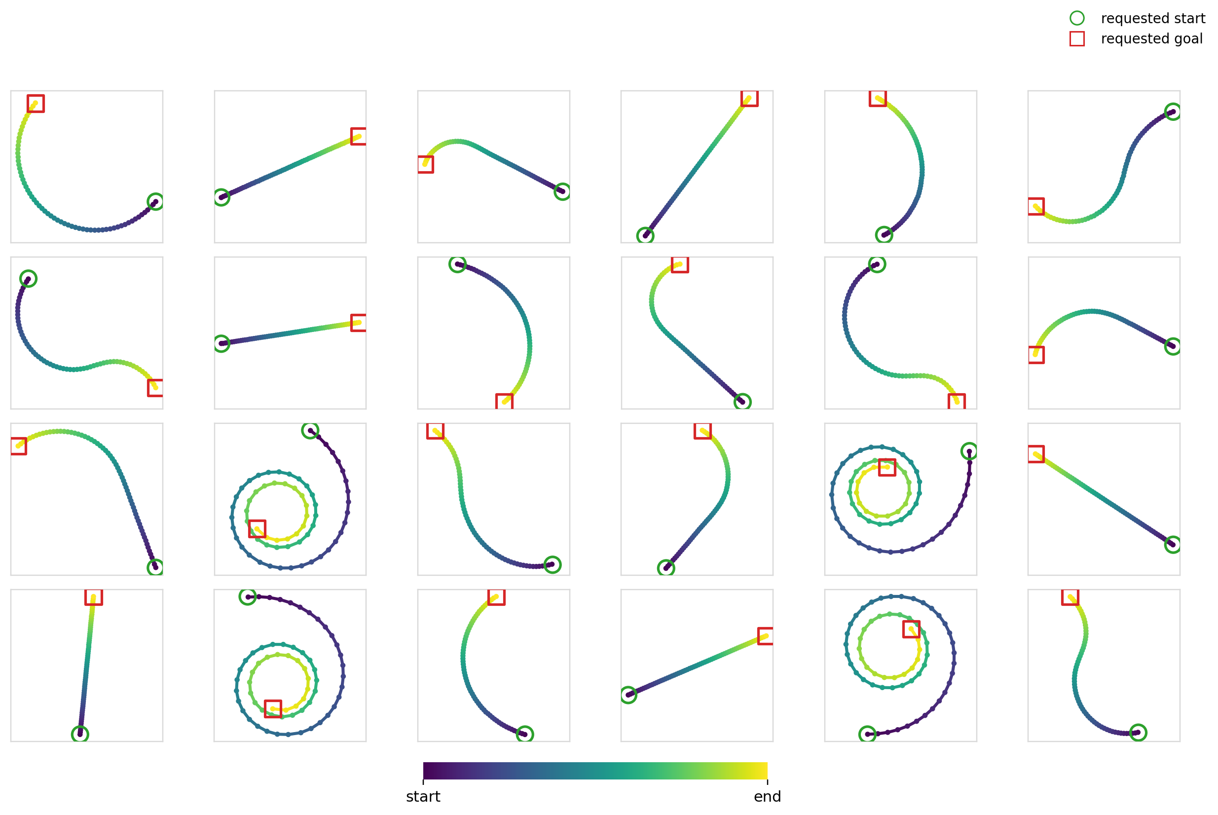
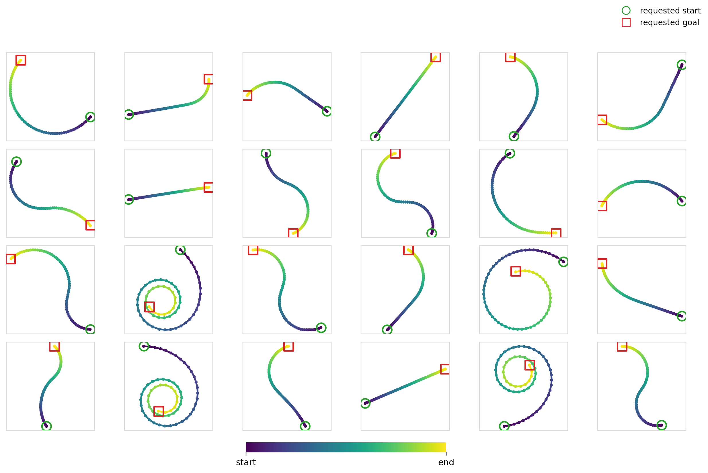
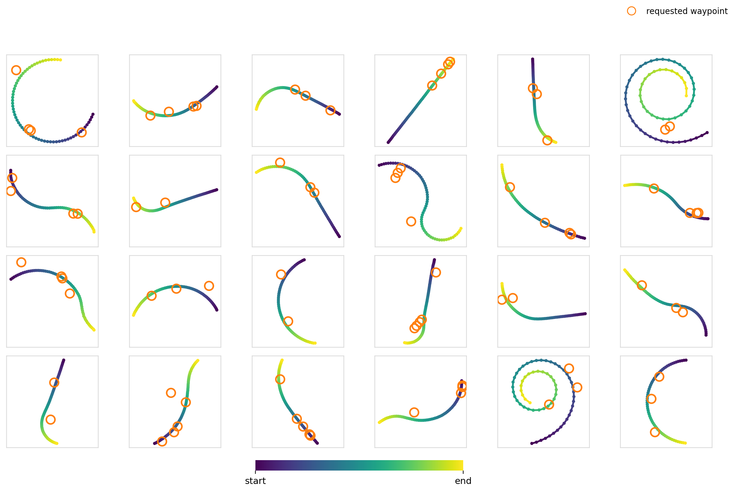
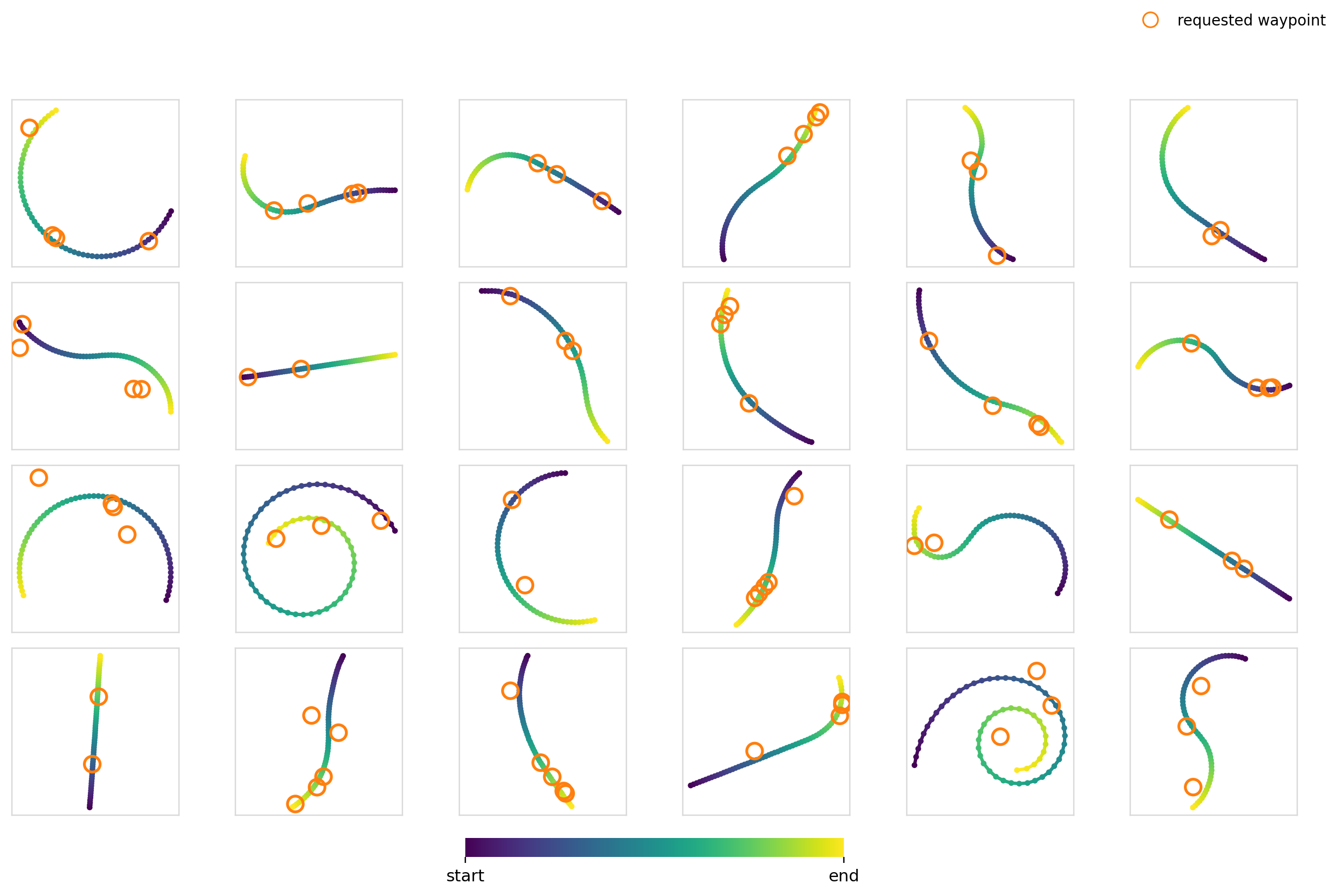
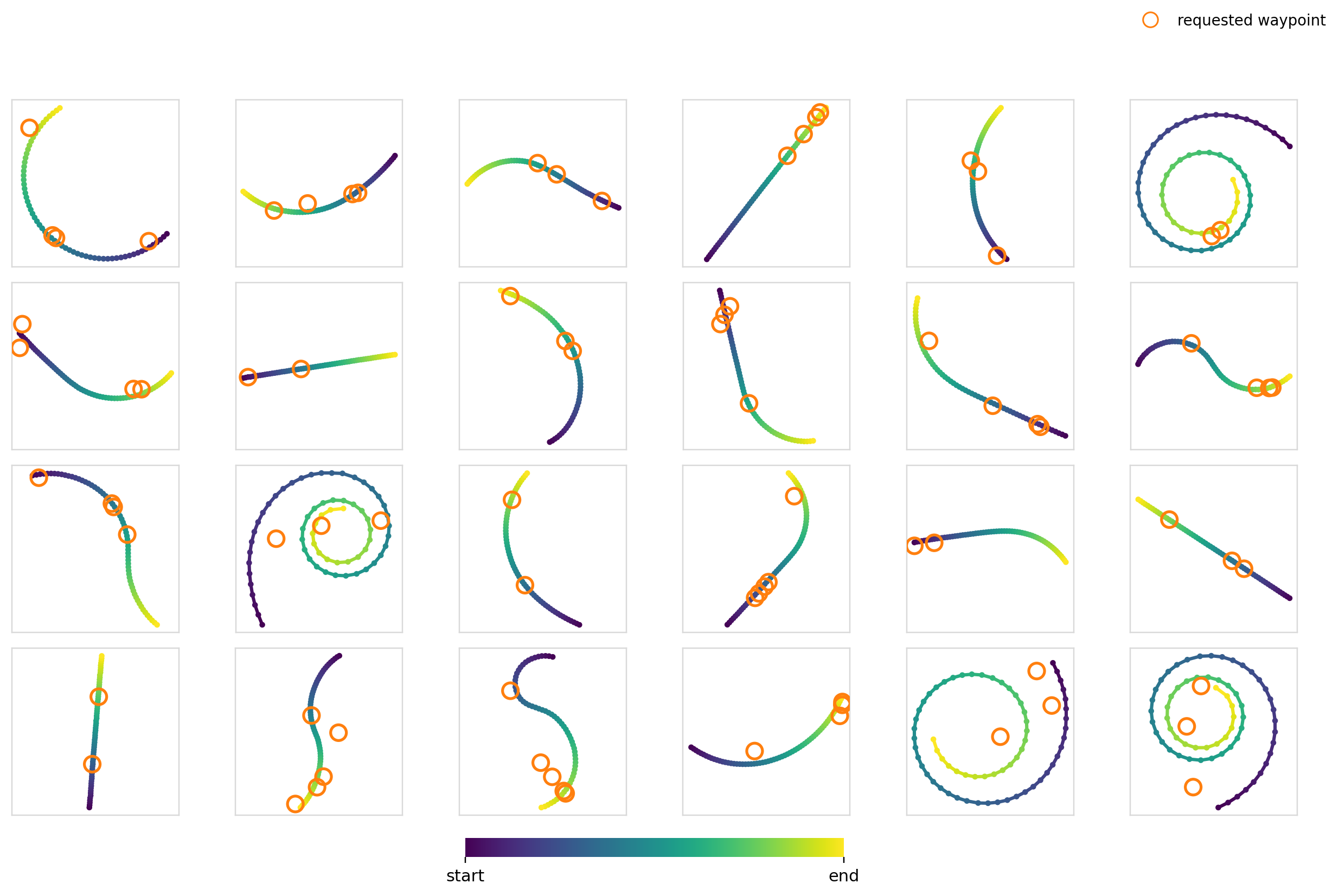
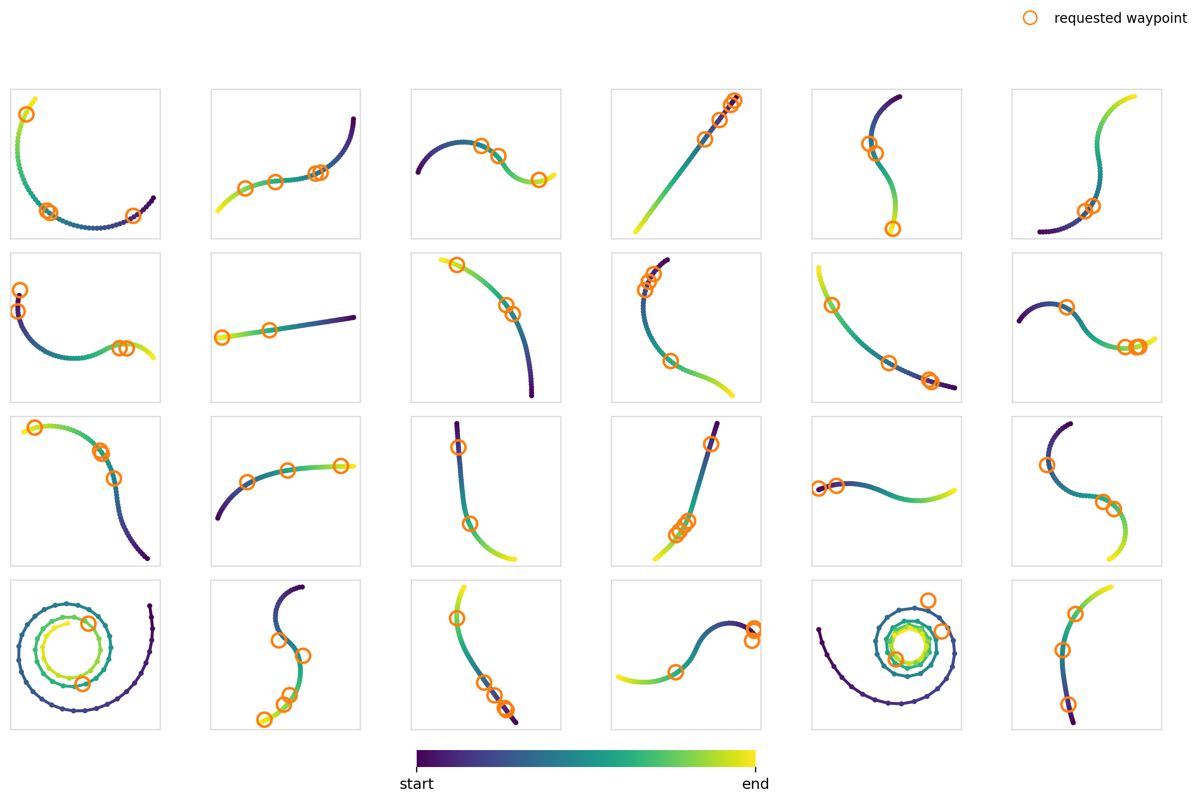
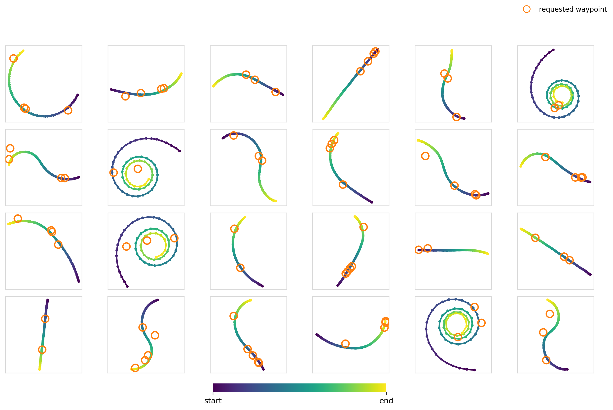
Now it’s time to really crank up the difficulty. For this experiment, we condition the model on a set of 2-5 waypoints with the restriction that the trajectory must pass through them. For the training data, we just randomly sample 2-5 points on trajectories in the dataset.
For the global mechanisms, we stack each of the waypoints and zero pad to hit the max number of points. This leaves us with a dim=10 vector. For cross-attention, we cross attend between each of the waypoint tokens and the action timesteps.
I thought this would be difficult for a few reasons:
- The number of waypoints isn’t constant. The model has to learn to be combination invariant for maximum effectiveness
- It constrains specific parts of the trajectory, but moreover makes the model choose where the constraint needs to be applied through trying to generate a trajectory in the data distribution
Surely FiLM completely breaks apart here right?
| Diffusion | Flow Matching | |
|---|---|---|
| FiLM | 0.5261 | 0.7166 |
| AdaGN | 0.5620 | 0.6584 |
| Concat | 0.6189 | 0.6995 |
| Cross-attn | 0.8845 | 0.8596 |
Here we measure the hit-rate as a fraction of waypoints with a trajectory point with . The values were computed over 3,840 samples per model x mechanism pair.
Some more metrics before we try to make sense of the results:
| Hit-rate | Mean dist | Diversity | Class Entropy | |
|---|---|---|---|---|
| Diffusion + FiLM | 0.526 | 0.0671 | 6.907 | 0.673 |
| Diffusion + AdaGN | 0.562 | 0.0616 | 6.909 | 0.658 |
| Diffusion + Concat | 0.619 | 0.0550 | 6.922 | 0.651 |
| Diffusion + Cross-attn | 0.884 | 0.0264 | 6.853 | 0.627 |
| Flow Matching + FiLM | 0.717 | 0.0441 | 6.525 | 0.542 |
| Flow Matching + AdaGN | 0.658 | 0.0516 | 6.632 | 0.603 |
| Flow Matching + Concat | 0.700 | 0.0464 | 6.397 | 0.561 |
| Flow Matching + Cross-attn | 0.860 | 0.0289 | 6.352 | 0.539 |
Mean distance is just the average of the closest distances between the waypoints and points on the trajectory. Class entropy is a measure of how many classes the model samples are spread across. (We use the Oracle to estimate this).
The things that stood out to me are:
- Hit-rates are pretty low in general. Either this is a pretty difficult task, or I didn’t do a good enough job at designing and training the model. I’d wager it’s a combination of both
- The global mechanisms’ hit-rates are unreasonably high. You don’t just hit
>50%of waypoints by guessing - There isn’t any difference between the individual global conditioning mechanisms (Except for maybe the diffusion + concatenation combination compared to other diffusion combinations. This might be due to the combinatorial nature of the problem)
- Flow matching handily beats diffusion when coupled with global conditioning mechanisms. This isn’t just statistical noise
- As expected cross-attention performs the best here as it can make use of timestep specific conditioning. It also produces the best mean distance metrics. It still doesn’t crack the
90%hit-rate, probably due to the factors mentioned above. I’m sure it’s possible to tune the model and training parameters to get this number a lot higher - Diversity metrics are the similar across all configurations, maybe slightly lower for the flow matching configurations
- Class entropy is also similar, maybe a bit lower for the flow matching configurations
Trying to reason about these:
- The global mechanisms are probably doing some sort of “shape-fitting”, matching waypoint configurations to high level trajectory shapes. The way these mechanisms propagate conditioning information isn’t conducive to handling waypoint binding constraints, but it doesn’t mean that they’re completely helpless either
- The flow matching disparity is also very interesting. We can perhaps chalk some of it to the fact that it produces trajectories with slightly lower diversity and entropy scores. The question is why?
- Flow matching 2 uses a schedule to sample
tunlike diffusion that samplestuniformly. Maybe this was a bad comparison and I should’ve made these symmetric, but as they say, it’s impossible to appreciate symmetry if there isn’t any asymmetry to juxtapose against. - Here’s something a bit more speculative: Diffusion’s SNR weighted loss could be diminishing conditioning gradients at high
t(higher noise levels), compared to flow matching’s velocity prediction. This does make sense if we think of the global mechanisms solving this problem by “shape-fitting” and making high level decisions. Making high level decisions at hightthat decide the success rate of the task probably suits flow matching more. The conditioning mechanisms don’t allow for lowtrefinement either. This would also explain why there isn’t much of a difference between the two when it comes to cross-attention
- Flow matching 2 uses a schedule to sample
The above metrics were all obtained on inputs that were “in distribution”, meaning that the waypoints were sampled from trajectories in the dataset. Doing it this way makes it so that there is always a feasible trajectory that threads the points, but may also introduce some bias. I also ran some OOD evaluations to check if that would tell us something more. (To be perfectly fair the bias angle isn’t particularly real given that our spatial domain is small and bounded, and the training sample covers most of it anyway. The joint distribution of the waypoints should also be amply covered by the original dataset).
I took in-distribution waypoint samples and slowly added gaussian noise to them (parameterized by ). So corresponds to the previous setup and the waypoints get increasingly random as we move down the rows.
| Sigma | FiLM | AdaGN | Concat | Cross-attn |
|---|---|---|---|---|
| 0.000 | 0.5312 | 0.5340 | 0.5798 | 0.8214 |
| 0.036 | 0.4715 | 0.4994 | 0.5402 | 0.7673 |
| 0.071 | 0.3689 | 0.4219 | 0.4459 | 0.6674 |
| 0.107 | 0.3521 | 0.3661 | 0.4118 | 0.6010 |
| 0.143 | 0.2997 | 0.2997 | 0.3845 | 0.5491 |
| 0.179 | 0.2740 | 0.2801 | 0.3248 | 0.4883 |
| 0.214 | 0.2461 | 0.2824 | 0.3326 | 0.4710 |
| 0.250 | 0.2628 | 0.2489 | 0.2935 | 0.4715 |
| 0.286 | 0.2282 | 0.2433 | 0.2824 | 0.4648 |
| 0.321 | 0.2260 | 0.2405 | 0.2746 | 0.4637 |
| 0.357 | 0.2294 | 0.2433 | 0.2924 | 0.4431 |
| 0.393 | 0.2400 | 0.2277 | 0.2796 | 0.4308 |
| 0.429 | 0.2048 | 0.2254 | 0.2528 | 0.4163 |
| 0.464 | 0.2221 | 0.2221 | 0.2656 | 0.4107 |
| 0.500 | 0.1931 | 0.2065 | 0.2506 | 0.4057 |
| Sigma | FiLM | AdaGN | Concat | Cross-attn |
|---|---|---|---|---|
| 0.000 | 0.6602 | 0.6110 | 0.6652 | 0.8270 |
| 0.036 | 0.5586 | 0.5871 | 0.5921 | 0.7640 |
| 0.071 | 0.4833 | 0.4397 | 0.4967 | 0.6233 |
| 0.107 | 0.4280 | 0.3811 | 0.4146 | 0.5312 |
| 0.143 | 0.3739 | 0.3538 | 0.3984 | 0.5151 |
| 0.179 | 0.3594 | 0.3287 | 0.3287 | 0.4637 |
| 0.214 | 0.3320 | 0.2946 | 0.3103 | 0.4487 |
| 0.250 | 0.3348 | 0.3158 | 0.3164 | 0.4615 |
| 0.286 | 0.3147 | 0.2919 | 0.3069 | 0.4386 |
| 0.321 | 0.3153 | 0.2829 | 0.2829 | 0.3996 |
| 0.357 | 0.2902 | 0.2768 | 0.2868 | 0.4012 |
| 0.393 | 0.2974 | 0.2679 | 0.2902 | 0.4202 |
| 0.429 | 0.3075 | 0.2634 | 0.2919 | 0.3906 |
| 0.464 | 0.2846 | 0.2288 | 0.2556 | 0.3968 |
| 0.500 | 0.2807 | 0.2360 | 0.2734 | 0.3772 |
There’s a lot to process here, and this is admittedly not the most sound of experiments. But we’ll work with what we have. The hit-rates drop as the inputs get more random, which is expected. The problem is that a good % of these probably don’t even have a feasible solution that can thread all of the waypoints. The one saving grace is that the hit-rate counts the fraction of waypoints hit and isn’t binary for the trajectory. This means that it’s always possible to hit at least one waypoint for a given set of waypoints. So this basically becomes a contest of which method can make the best out of the random inputs. You might ask why I didn’t just sample another dataset for the OOD waypoints. That would mean that I wouldn’t be able to evaluate on noise injected inputs, which was a bit too thematic to resist.
To make some sense of this, we look at the retention, which is the % of hit-rate that is preserved as we go from to
| Cross-attn retention | Trio retention | |
|---|---|---|
| Diffusion | 49.4% | 39.5% |
| Flow Matching | 45.6% | 40.8% |
We see that cross-attention retains more of its hit-rate as the waypoints get more infeasible. This reinforces the fact that cross-attention does a better job at solving this task and is more robust to noise in the distribution of waypoints.
Experiment 5
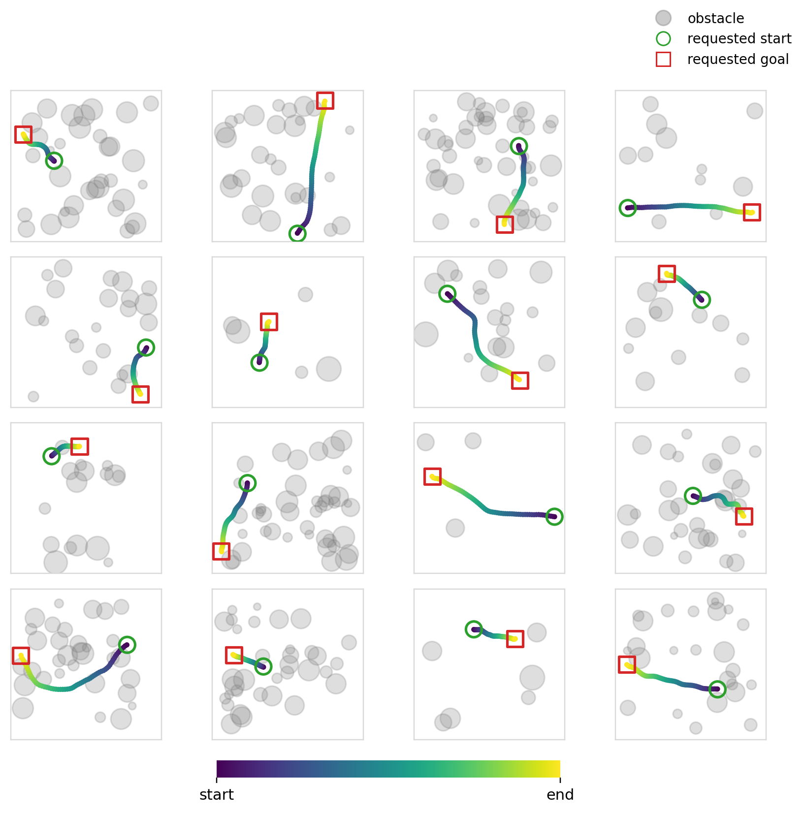
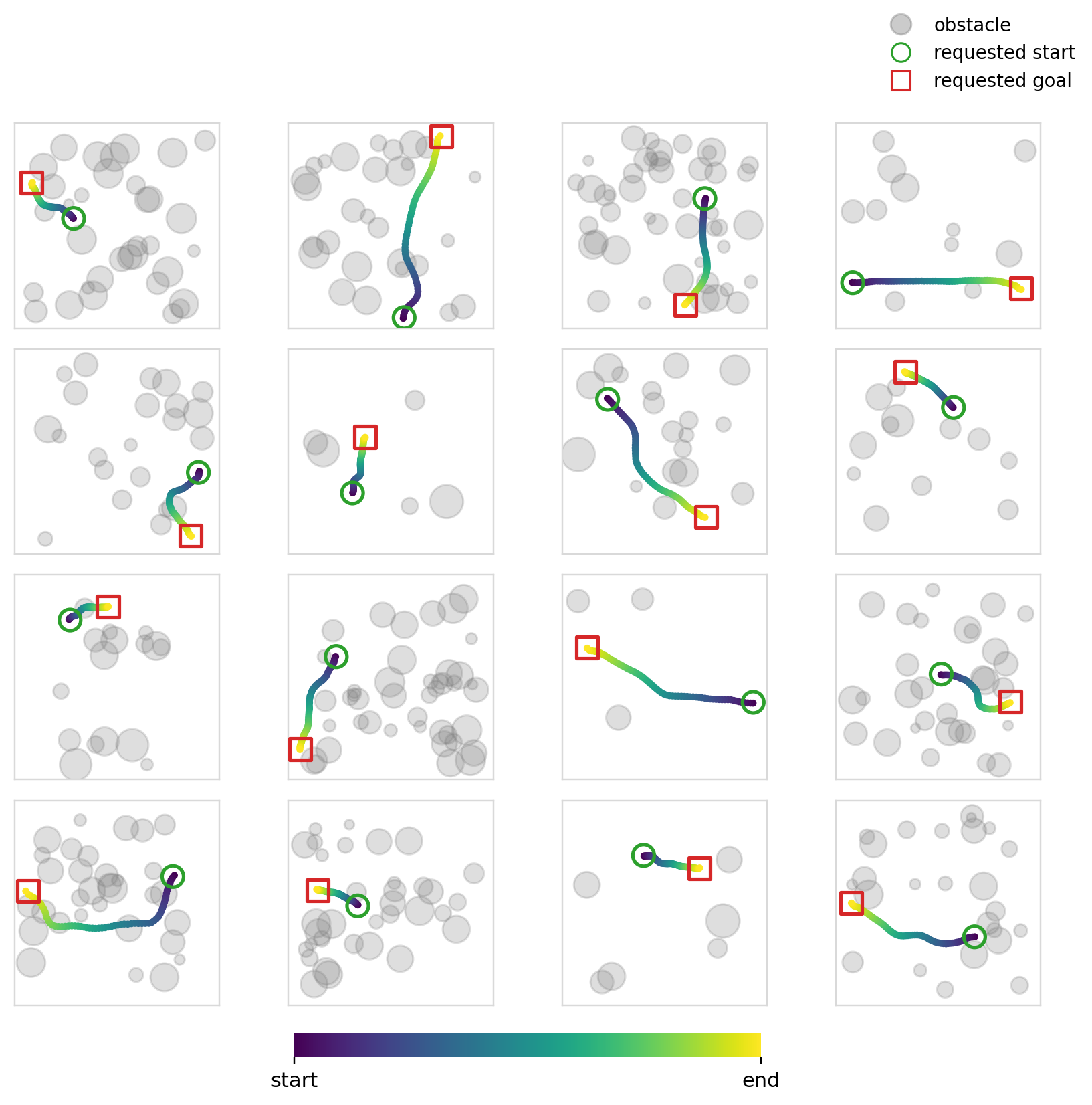
The first “experiment 5” had me try to do obstacle avoidance with Dataset1. Let’s just say that neither the setup, nor the eval made any sense (for obvious reasons), so we can pretend that it never happened. The real experiment uses dataset2.
| Policy | Steps | Batch | LR | NFE |
|---|---|---|---|---|
| Diffusion | 7k | 1536 | 2.5e-4 | 50 |
| Flow Matching | 7k | 1536 | 2.5e-4 | 20 |
| FiLM | AdaGN | Concat | Cross-attn |
|---|---|---|---|
| 12.298 | 12.298 | 11.358 | 12.593 |
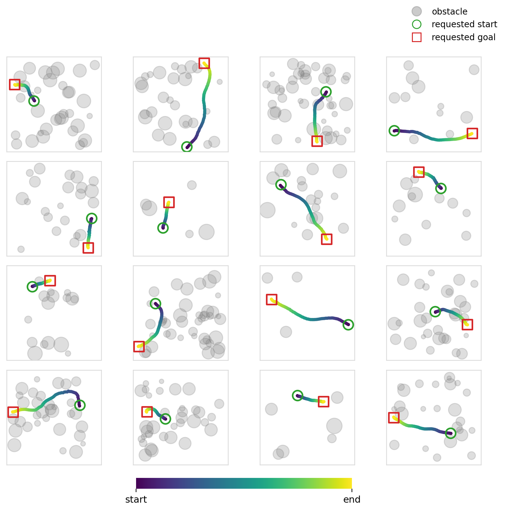
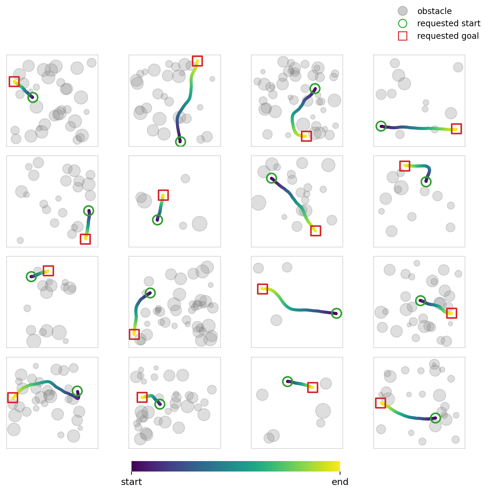
The objective of this experiment (and the next) is fairly simple: learn collision free trajectories in an occupancy map. We use Dataset2 (See Dataset for details) and train policies to output feasible trajectories. This problem specifically requires a high degree of local action conditioning in order to produce samples with a high success rate. Global conditioning methods, in theory, shouldn’t be able to solve this problem well as they don’t have localized control of the actions at the level that is required.
For this specific experiment, we try something similar to what is usually done with image inputs to such models. We encode the occupancy map and endpoints into one dim=128 vector and condition every mechanism using this single vector. We use ResNet 11 style CNN blocks to encode the image. Cross-attention is also made to use the same vector across all of the timesteps.
| Diffusion | Flow Matching | |
|---|---|---|
| FiLM | 0.5430 | 0.5195 |
| AdaGN | 0.5391 | 0.5312 |
| Concat | 0.5488 | 0.5098 |
| Cross-attn | 0.5215 | 0.5059 |
| Diffusion | Flow Matching | |
|---|---|---|
| FiLM | 0.4570 | 0.4805 |
| AdaGN | 0.4609 | 0.4688 |
| Concat | 0.4512 | 0.4902 |
| Cross-attn | 0.4785 | 0.4941 |
| Diffusion | Flow Matching | |
|---|---|---|
| FiLM | 0.0068 | 0.0097 |
| AdaGN | 0.0076 | 0.0106 |
| Concat | 0.0055 | 0.0092 |
| Cross-attn | 0.0069 | 0.0094 |
During evaluation, we sample 512 configurations (occupancy map + endpoints) and evaluate each model-mechanism pair on these. The occupancy maps are sampled using the same sparse, medium, dense split as during dataset creation.
The models solve the endpoint constraints pretty well. We’ve already established that global mechanisms have no difficulty with this, so this shouldn’t come as a surprise. We also measure the collision rate and the success rate. The collision rate is the fraction of samples whose minimum signed distance to any obstacle in the map is < 0. The success rate is the fraction of samples that are both collision free and within the endpoint error of 0.05.
The success and collision rates are modest, no doubt being propped up by the sparse samples. Cross-attention is better in terms of collision and success rates, but the difference isn’t that large. All four mechanisms perform similarly as expected. Flow matching continues to perform better (though the margin is smaller this time), perhaps hinting again at its effectiveness when paired with global conditioning methods.

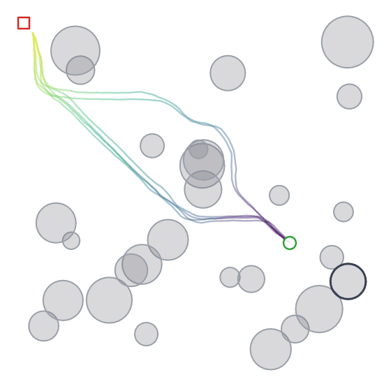
Experiment 6
| Policy | Steps | Batch | LR | NFE |
|---|---|---|---|---|
| Diffusion | 30k | 2560 | 3.2e-4 | 50 |
| Flow Matching | 30k | 2560 | 3.2e-4 | 20 |
| FiLM | AdaGN | Concat | Cross-attn |
|---|---|---|---|
| 35.396 | 35.396 | 34.522 | 34.949 |
For this final experiment, we try our best to solve the problem. Instead of generating a single feature vector, we encode the image ViT style 12 using 8x8 patches and a hidden dimension of 128. For the global mechanisms, these patch tokens and the endpoint tokens are stacked and used for conditioning. For cross-attention, we take the input tokens and compute cross-attention with all of the action timesteps.
(Note that I also tried a 4x4 patch version with a smaller hidden dimension where cross-attention still performed better than the global methods but not nearly as decisively as in this experiment).
| Metric | Diffusion | Flow Matching | ||||||
|---|---|---|---|---|---|---|---|---|
| FiLM | AdaGN | Concat | Cross-attn | FiLM | AdaGN | Concat | Cross-attn | |
| Success rate ↑ | 0.576 | 0.570 | 0.557 | 0.959 | 0.551 | 0.549 | 0.525 | 0.916 |
| Collision rate ↓ | 0.424 | 0.430 | 0.443 | 0.041 | 0.449 | 0.451 | 0.475 | 0.084 |
| Endpoint error ↓ | 0.0057 | 0.0060 | 0.0034 | 0.0020 | 0.0066 | 0.0084 | 0.0050 | 0.0034 |
| Success · sparse ↑ | 0.851 | 0.862 | 0.851 | 1.000 | 0.851 | 0.872 | 0.851 | 1.000 |
| Success · medium ↑ | 0.692 | 0.654 | 0.654 | 0.995 | 0.670 | 0.637 | 0.632 | 0.973 |
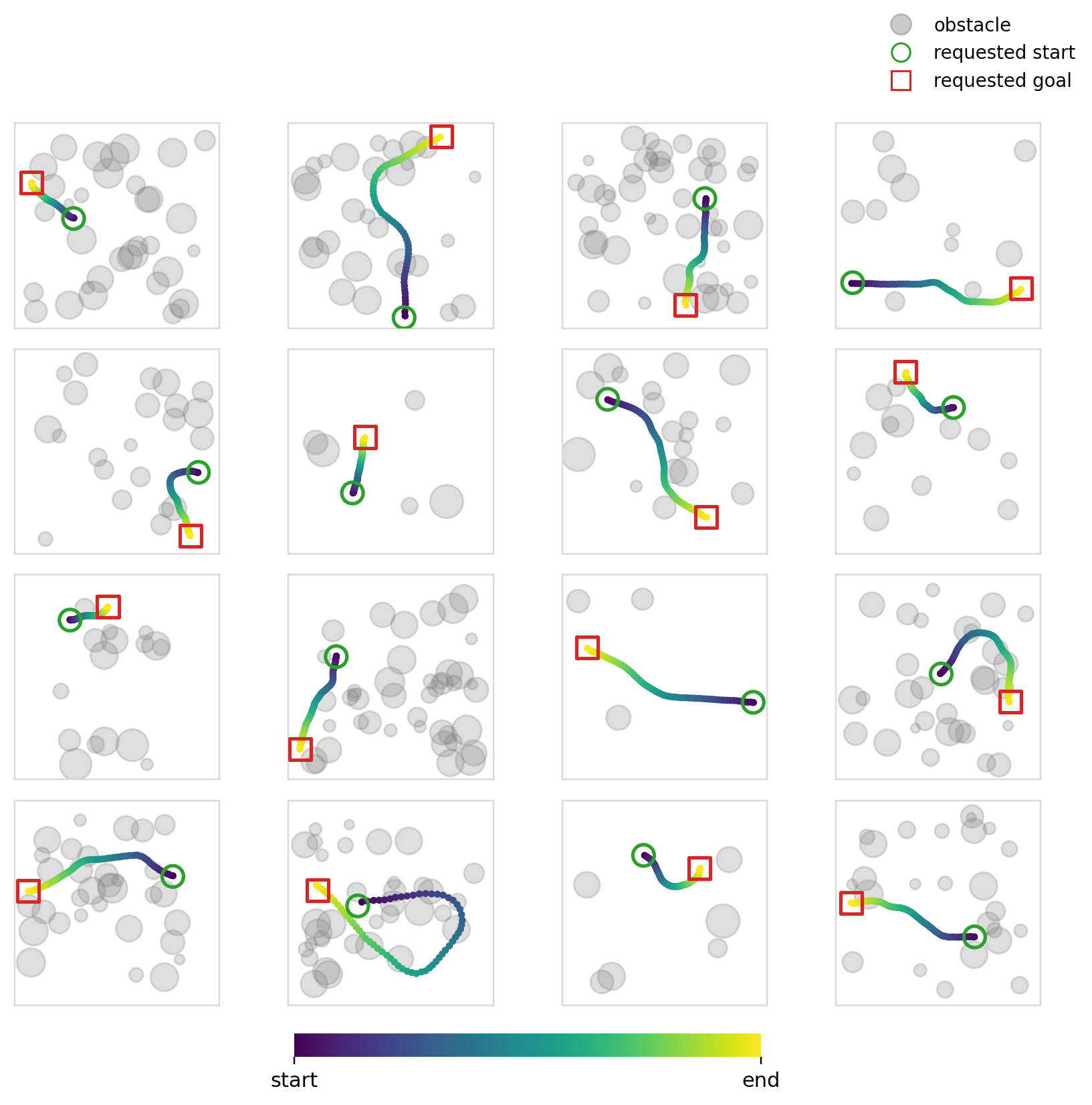
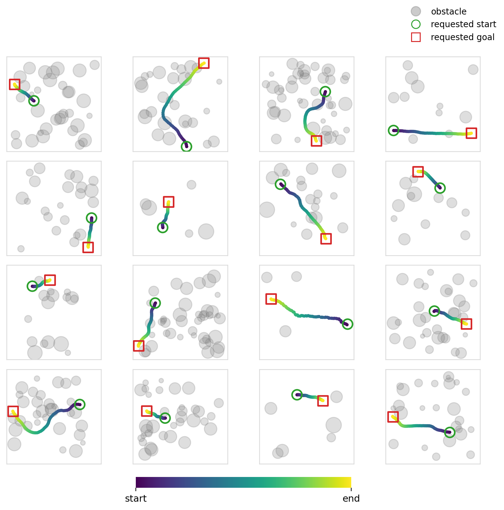
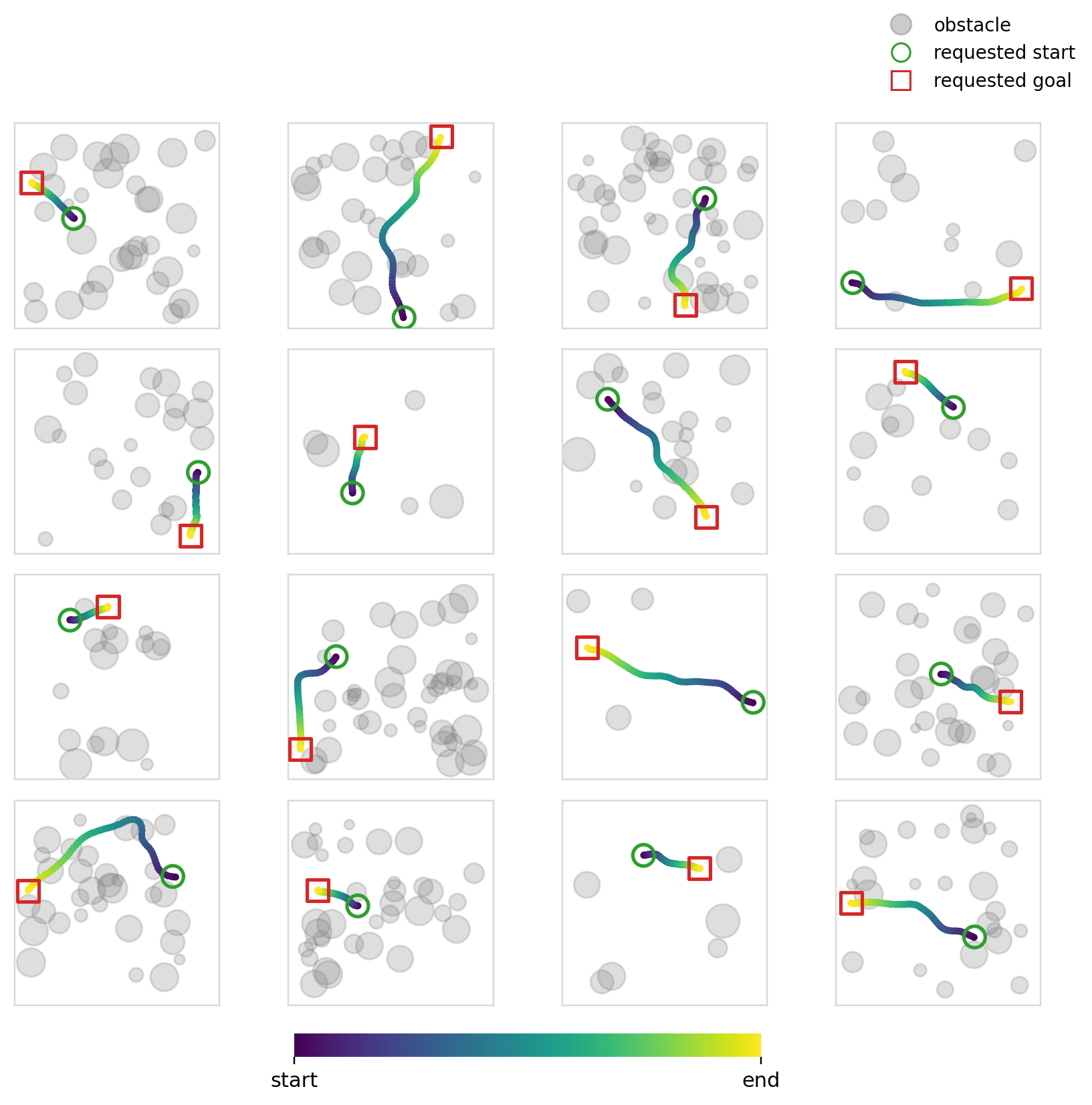
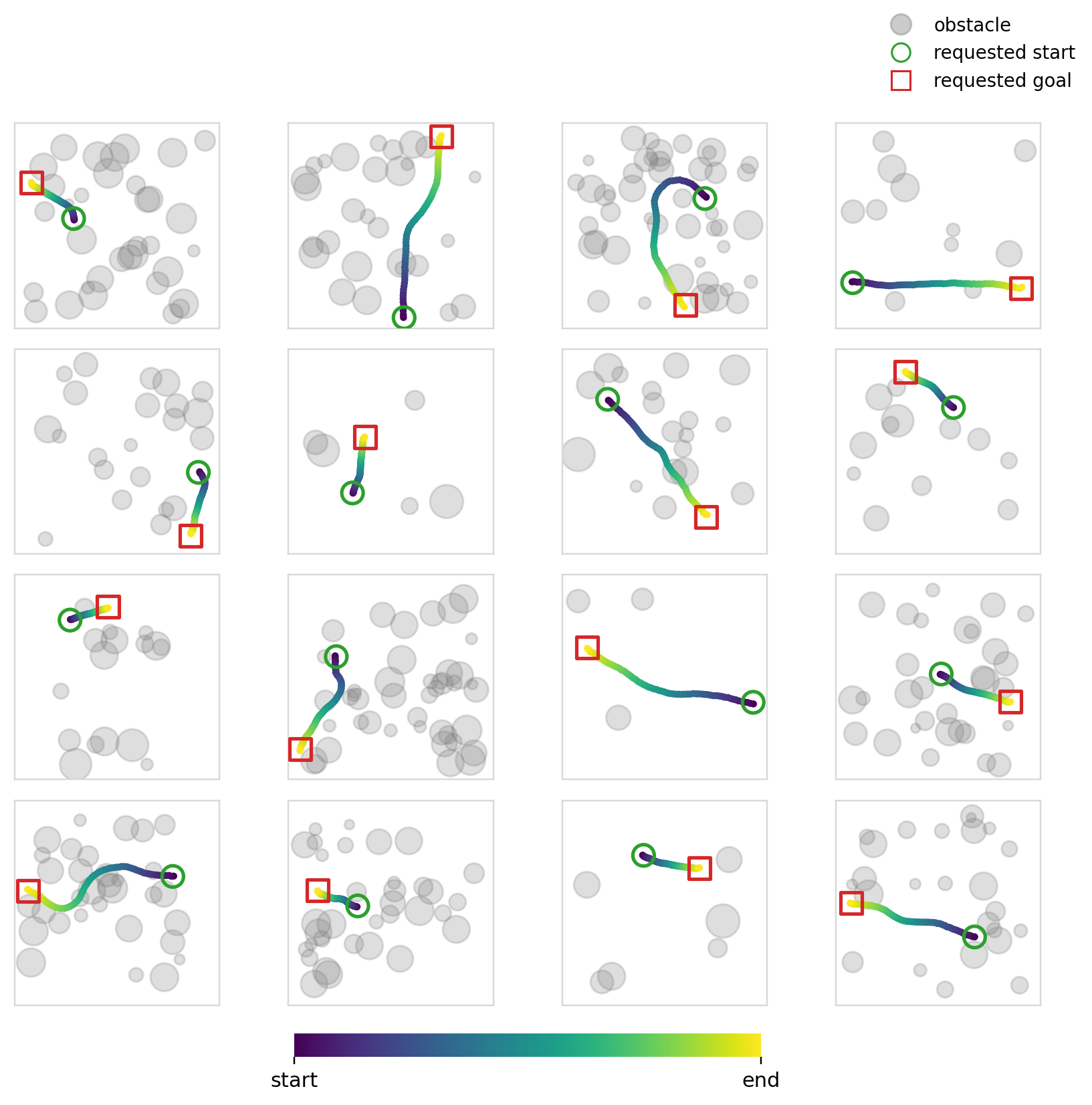
| Success · dense ↑ | 0.377 | 0.390 | 0.364 | 0.915 | 0.339 | 0.352 | 0.314 | 0.839 |
As expected, cross-attention dominates the field here. Its success rate on dense occupancy maps isn’t perfect, probably due to a mixture of the problem being difficult and the model and training process not being optimized enough. Interestingly, flow matching performs slightly to moderately worse in most configurations. I’m not sure why. It could be something to do with the model or training process. Going back to our previous theoretical reasoning, it could also be because flow matching tries to do more at the initial noisy steps, leading to more unstable steps when working with high information conditioning features. Running an experiment without the time-samping asymmetry might shed some more light here, but it isn’t something I’ve tested yet.
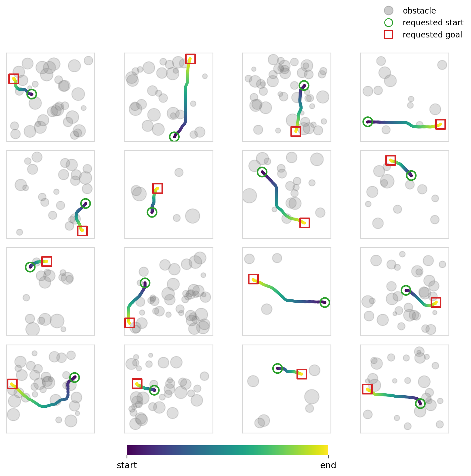
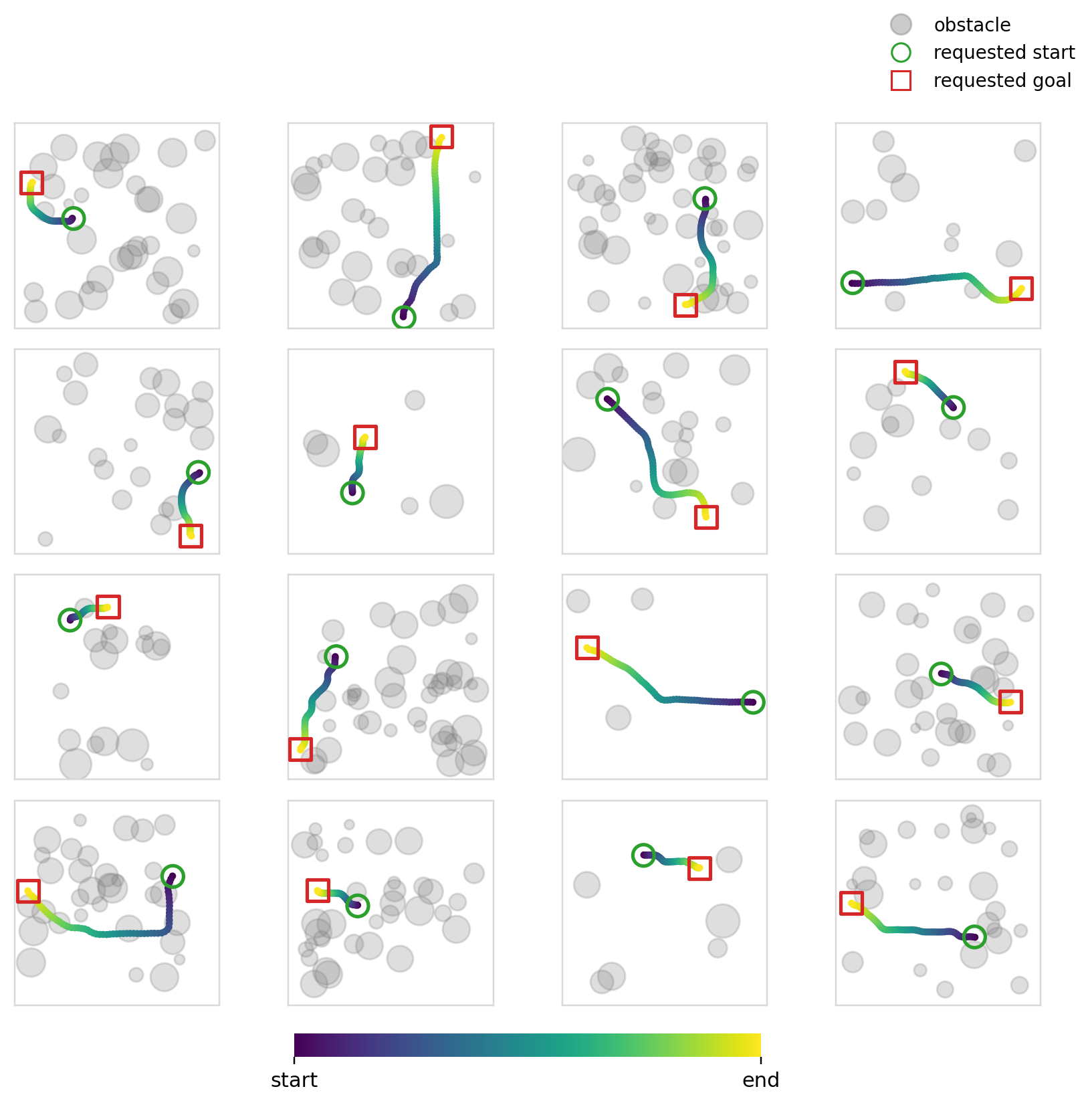


Below we can see the samples that the model (diffusion + cross-attention) produces. We can also see its multi-modality in action (although in this case you could argue that it isn’t ideal given that it was trained to reproduce shortest distance paths).
Takeaways
So what did we learn?
- There isn’t really that much difference between the three global mechanisms. FiLM and AdaGN are pretty interchangeable. Simple concatenation proved to be effective as well, but for more complex policies we’d probably have an easier time training with some modulation mechanism
- Global mechanisms have no business being this effective. They tend to do well even on problems that might seem too difficult for them at first glance. If you had to choose a conditioning mechanism for your policy, FiLM should probably be your first choice
- Flow matching seems to be the better generative model when it comes to making the best out of limited resources (global conditioning on difficult tasks). It also needs fewer denoising steps, making it a good default for a lot of tasks. Some effects with flow matching probably still need to be investigated further
- Use global conditioning when you just need high level decision making or need to satisfy high level constraints. Use cross-attention when you need more local control over your actions. Of course, if you’re using a DiT backbone 9, cross-attention becomes the natural choice
References
References
-
Perez, E., Strub, F., de Vries, H., Dumoulin, V., & Courville, A. (2018). FiLM: Visual reasoning with a general conditioning layer. In Proceedings of the AAAI Conference on Artificial Intelligence (Vol. 32, No. 1). [Link] ↩ ↩2
-
Lipman, Y., Chen, R. T. Q., Ben-Hamu, H., Nickel, M., & Le, M. (2023). Flow matching for generative modeling. In International Conference on Learning Representations (ICLR). [Link] ↩ ↩2 ↩3
-
Vaswani, A., Shazeer, N., Parmar, N., Uszkoreit, J., Jones, L., Gomez, A. N., Kaiser, L., & Polosukhin, I. (2017). Attention is all you need. Advances in Neural Information Processing Systems, 30, 5998-6008. [Link] ↩ ↩2
-
Chi, C., Xu, Z., Feng, S., Cousineau, E., Du, Y., Burchfiel, B., Tedrake, R., & Song, S. (2023). Diffusion policy: Visuomotor policy learning via action diffusion. In Proceedings of Robotics: Science and Systems (RSS). [Link] ↩ ↩2
-
Ho, J., Jain, A., & Abbeel, P. (2020). Denoising diffusion probabilistic models. Advances in Neural Information Processing Systems, 33, 6840-6851. [Link] ↩
-
Nichol, A., & Dhariwal, P. (2021). Improved denoising diffusion probabilistic models. In Proceedings of the 38th International Conference on Machine Learning (pp. 8162-8171). PMLR. [Link] ↩
-
Song, J., Meng, C., & Ermon, S. (2021). Denoising diffusion implicit models. In International Conference on Learning Representations (ICLR). [Link] ↩
-
Black, K., Brown, N., Driess, D., Esmail, A., Equi, M., Finn, C., Fusai, N., … & Zhilinsky, U. (2025). π0: A vision-language-action flow model for general robot control. In Proceedings of Robotics: Science and Systems (RSS). [Link] ↩
-
Peebles, W., & Xie, S. (2023). Scalable diffusion models with transformers. In Proceedings of the IEEE/CVF International Conference on Computer Vision (pp. 4172-4182). [Link] ↩ ↩2
-
Dhariwal, P., & Nichol, A. (2021). Diffusion models beat GANs on image synthesis. Advances in Neural Information Processing Systems, 34, 8780-8794. [Link] ↩
-
He, K., Zhang, X., Ren, S., & Sun, J. (2016). Deep residual learning for image recognition. In Proceedings of the IEEE Conference on Computer Vision and Pattern Recognition (CVPR) (pp. 770-778). [Link] ↩
-
Dosovitskiy, A., Beyer, L., Kolesnikov, A., Weissenborn, D., Zhai, X., Unterthiner, T., Dehghani, M., Minderer, M., Heigold, G., Gelly, S., Uszkoreit, J., & Houlsby, N. (2021). An image is worth 16x16 words: Transformers for image recognition at scale. In International Conference on Learning Representations (ICLR). [Link] ↩
Comments