In this post, we take a look at this $[1]$ paper, which introduces a simple, yet interesting approach to solving a multi-vehicle path planning problem.
My implementation of the algorithm that was used to evaluate its performance and generate all the results in this post can be found here
$\newcommand{\ith}{i^{th}}$ $\newcommand{\pth}{p^{th}}$ $\newcommand{\qth}{q^{th}}$ $\newcommand{\lth}{l^{th}}$ $\newcommand{\MR}{\mathbb{R}}$ $\newcommand{\xpi}{x_{pi}}$ $\newcommand{\ypi}{y_{pi}}$ $\newcommand{\xqi}{x_{qi}}$ $\newcommand{\yqi}{y_{qi}}$ $\newcommand{\xmin}{x_{min}}$ $\newcommand{\xmax}{x_{max}}$ $\newcommand{\ymin}{y_{min}}$ $\newcommand{\ymax}{y_{max}}$ $\newcommand{\xlmin}{x_{l,min}}$ $\newcommand{\xlmax}{x_{l,max}}$ $\newcommand{\ylmin}{y_{l,min}}$ $\newcommand{\ylmax}{y_{l,max}}$ $\newcommand{\xlimin}{x_{li,min}}$ $\newcommand{\xlimax}{x_{li,max}}$ $\newcommand{\ylimin}{y_{li,min}}$ $\newcommand{\ylimax}{y_{li,max}}$ $\newcommand{\cplx}{c_{pl,x}}$ $\newcommand{\cply}{c_{pl,y}}$ $\newcommand{\dpqx}{d_{pq,x}}$ $\newcommand{\dpqy}{d_{pq,y}}$ $\newcommand{\tpli}{t_{pli}}$ $\newcommand{\spi}{s_{pi}}$ $\newcommand{\spij}{s_{pij}}$ $\newcommand{\spinext}{s_{p,i+1}}$ $\newcommand{\spn}{s_{pN}}$ $\newcommand{\spf}{s_{pf}}$ $\newcommand{\wpi}{w_{pi}}$ $\newcommand{\wpij}{w_{pij}}$ $\newcommand{\wpn}{w_{pN}}$ $\newcommand{\upi}{u_{pi}}$ $\newcommand{\upik}{u_{pik}}$ $\newcommand{\vpi}{v_{pi}}$ $\newcommand{\vpik}{v_{pik}}$ $\newcommand{\Ap}{A_{p}}$ $\newcommand{\Bp}{B_{p}}$ $\newcommand{\qp}{q_{p}}$ $\newcommand{\rp}{r_{p}}$ $\newcommand{\pp}{p_{p}}$
Problem
The paper tries to tackle the issue of finding fuel optimal paths for multiple vehicles, given vehicle-obstacle and vehicle-vehicle collision constraints. The paper being more than two decades old, makes this a rather interesting read because it comes from a time well before the advent of sophisticated trajectory optimization methods we see today.
The fuel optimal cost function is formulated as a linear program, with the collision constraints being represented as linear constraints using binary integer variables. The entire problem is thus cast as a Mixed Integer Program (MIP), and taking into account that it accounts for multiple vehicles, the rest of the post shall refer to the algorithm as MVMIP.
Formulation
Preliminaries
The planning problem under consideration is usually cast as an optimization problem with a quadratic cost.
\begin{equation} \begin{aligned} \min_{s, u}J = \min_{s, u}\int_{0}^{\infty}(s^TQs + u^TRu)dt\\ \text{s.t.} \ \ \dot{s} = As + Bu \end{aligned} \end{equation}
Where $s \in \MR^n$ represents the robot state and $u \in \MR^m$ represents the control input that need to be executed at each time step. $Q \in \MR^{n \times n}$ and $R \in \MR^{n \times m}$ are the cost matrices for the quadratic cost.
Due to the fact that we want to cast this as an MIP, this cost will be cast as a linear cost that looks like:
\begin{equation} \min_{s, u}J = \min_{s, u}\int_{0}^{\infty}(q^T|s| + r^T|u|)dt \end{equation}
Here $q \in \MR^n$ and $r \in \MR^m$ are cost vectors that form the linear equivalent of the quadratic cost. $|v|$ is a vector denoting the absolute values of the vector $v$ being operated on.
Objective
As is common in these scenarios, to make the problem tractable, it is discretized into $N$ time steps. Separate costs vectors are also introduced for the final state $s_N$. This is a familiar trope in planning and allows for greater flexibility in generating the results we need, which we will see later.
\begin{equation} \begin{aligned} \min_{s, u}J = \min_{s, u}\sum_{i=0}^{N-1}(q^T|s_i| + r^T|u_i|)\Delta t + f(s_N)\\ \text{s.t.} \ \ s_{i+1} = As_i + Bu_i \end{aligned} \end{equation}
$s_i$ and $u_i$ are the variables of the optimization and represent the robot’s trajectory and control inputs required to generate the state trajectory. Solving for these for each robot will essentially solve the MVMIP problem. $s_0$ is the initial state of the robot and is not a variable. $s_f$ denotes the expected or required final state of the robot. $u_0$ is the control input at the first time step and is a variable, but $u_N$ is not as we don’t expect to apply any control on the last step where the robot is expected to have reached $s_f$.
As mentioned, $q$ applies to each state vector $s_1$ through $s_{N-1}$, with $s_N$ having a corresponding cost term of $f(s_N)$
The objective as we see now tries to minimize the cost on the state and control. The minimum value for this objective is when both states and control inputs are zero but this is not what we desire. Driving the control inputs to zero is fine as we’re looking for fuel optimal paths, but driving the state also to zero is not the behavior we want as we’re not constructing a regulator.
Ideally we would want the state of the vehicle/robot to reach the final state $s_f$. So instead of driving the state to zero, we would like the problem to drive it to the required final state. This can easily be done by replacing $s_i$ with $s_i - s_f$ which makes it so that instead of driving $s_i \to 0$, we are driving $s_i - s_f \to 0$ which means driving $s_i \to s_f$.
And finally, we get to the multiple vehicle part of this whole thing, where we have states and control inputs for each required vehicle. The state and control of the $\pth$ vehicle will be represented as $\spi$ and the control input as $\upi$. The objective function for the $\pth$ vehicle is now (Note that some of the constant terms like $\Delta t$ can be ignored):
\begin{equation} J_p = \sum_{i=1}^{N-1}\qp^T|\spi - \spf| + \sum_{i=0}^{N-1}\rp^T|\upi| + \pp^T|\spn - \spf| \end{equation}
The question now is how does one frame this objective that has $|\ . |$ terms as a linear function with linear constraints? To answer this, we take a quick detour to go over a known result in linear programming.
Consider the following optimization problem: \begin{equation} \min_{x}q^T|x| \end{equation} Where $q, x \in \MR^n$. This can be written as: \begin{equation} \min_{x}\sum_{i=1}^{n}q_i |x_i| \end{equation} Where $|x_i|$ here is just the absolute value of the $\ith$ element of $x$.
We can now introduce slack variables $s_i$ for each $|x_i|$ such that $|x_i| \le s_i$ and frame the objective as a linear function in $s$. The objective will now be a minimization over $s$ and the constraint makes it so that minimizing $s$ will minimize each $|x_i|$ \begin{equation} \begin{aligned} \min_{x}\sum_{i=1}^{n}q_i x_i = \min_{s}q^Ts\\ \text{s.t.} \ \ |x_i| \le s_i \end{aligned} \end{equation} This is nice because it lets us keep a linear objective and represent the absolute inequality as two linear inequalities: \begin{equation} \begin{aligned} \min_{s}q^Ts\\ \text{s.t.} \ \ x_i \le s_i\\ -x_i \le s_i \end{aligned} \end{equation}
With this knowledge, we can now introduce slack variables $w$ and $v$ for $s$ and $u$ respectively. Representing the objective as an LP in these slack terms, along with taking the sum for every vehicle (assuming $K$ vehicles), we have the final objective function:
\begin{equation} \begin{aligned} \min_{w, v} \sum_{p=1}^{K}(\sum_{i=1}^{N-1}\qp^T\wpi + \sum_{i=1}^{N-1}\rp^T\vpi + \pp^T\wpn)\\ \text{s.t.} \ \ \spij - \spf \le \wpij\\ -\spij + \spf \le \wpij\\ \upik \le \vpik\\ -\upik \le \vpik\\ \spinext = \Ap\spi + \Bp\upi \end{aligned} \end{equation}
Note that we have the slack constraints for each element of the state and control vectors.
Vehicle-Obstacle Collision Constraints
Before we get to this, let’s take another detour to look at a concept that is something of a pre-requisite.
Let’s say we have an optimization problem of the form \begin{equation} \begin{aligned} \min_{x}f(x)\\ \text{s.t.} \ \ g_1(x) \le c_1\\ g_2(x) \le c_2\\ g_3(x) \le c_3\\ \vdots \end{aligned} \end{equation} Solving this would mean solving for the fact that ALL of the constraints need to be satisfied.
$g_1(x) \le c_1$ AND $g_2(x) \le c_2$ AND $g_3(x) \le c_3$, etc.
But what if we want don’t want each constraint to be satisfied? What if the our requirement is that at least one of them be active?
$g_1(x) \le c_1$ OR $g_2(x) \le c_2$ OR $g_3(x) \le c_3$, etc.
In this case, we can use a variant of the big-M method to help reframe the constraints. First we introduce binary integer variables $b_i \in \set{0, 1}$ for each constraint. We also introduce a constant $M$ that is an extremely large number relative to the range of the $g_i$ functions. The constraints can then be written as: \begin{equation} \begin{aligned} g_1(x) \le c_1 + Mb_1\\ g_2(x) \le c_2 + Mb_2\\ g_3(x) \le c_3 + Mb_3\\ \vdots\\ g_n(x) \le c_n + Mb_n\\ \sum_{i=1}^nb_i \le n-1 \end{aligned} \end{equation} Let’s dissect what’s happening here. Each $b_i$ can be either 0 or 1.
if a particular $b_i = 1$ (for the $\ith$ constraint), we have: \begin{equation} g_1(x) \le c_1 + M\\ \end{equation} And given that $M \gg g_1(x)$, this constraint will always be satisfied, irrespective of the value of $x$. if a particular $b_i = 0$, we have: \begin{equation} g_1(x) \le c_1\\ \end{equation} Which is just the original constraint.
So if $b_i = 1, \forall i \in \set{1, \ldots n}$, then this means that each constraint would trivially be satisfied, so this would be equivalent to not having any constraints at all.
On the other hand if $b_i = 0, \forall i \in \set{1, \ldots n}$, then then problem will be treated as an optimization problem where each of the original constraints need to be satisfied.
What happens if at least one of the $b_i$ values are restricted to be $0$? This would mean that at least one of the constraints (the ones where $b_i = 0$) will need to be satisfied (active), but the rest wouldn’t need to be active as they would be trivially satisfied due to $M$.
Hence by having an additional constraint on the sum of $b_i$ values, restricting them to a maximum value of $n-1$, we can guarantee that at least one $b_i = 0$. This then translates to our desired property of the optimization problem requiring only one of the constraints to be satisfied!
Equipped with this, we can now look at how the paper frames collision avoidance constraints. It is assumed that each obstacle is rectangular and the vehicle moves in a two dimensional space (It can easily be extended to 3D). Each vehicle/robot is also assumed to be a point.
If $s_i$ is the current state of the vehicle, we assume that the state contains some $x_i$ and $y_i$, which correspond to the $x$ and $y$ coordinates of the vehicle in 2D space. If the mid point of the obstacle is $(x_c, y_c)$ and its size is $(d_x, d_y)$, we can compute the bottom left and top right points as: \begin{equation} \begin{aligned} \xmin = x_c - 0.5d_x\\ \ymin = y_c - 0.5d_y\\ \xmax = x_c + 0.5d_x\\ \ymax = y_c + 0.5d_y\\ \end{aligned} \end{equation}
The vehicle at $(x_i, y_i)$ will avoid the obstacle (not be in collision) iff: \begin{equation} \begin{aligned} x_i \le \xmin\\ \text{OR} \ \ x_i \ge \xmax\\ \text{OR} \ \ y_i \le \ymin\\ \text{OR} \ \ y_i \ge \ymax\\ \end{aligned} \end{equation}
We require at least one of these constraints to be true. So we can use the big-M method to reframe these constraints!
\begin{equation} \begin{aligned} x_i \le \xmin + Mt_{i1}\\ -x_i \le -\xmax + Mt_{i2}\\ y_i \le \ymin + Mt_{i3}\\ -y_i \le -\ymax + Mt_{i4}\\ \sum_{k=1}^4t_{ik} \le 3 \end{aligned} \end{equation}
These constraints ensure that the vehicle avoids the obstacle, but offers no additional clearance from it. It also does not account for the vehicle itself having volume. In order to account for these, we can add additional clearance terms $c_x$ and $c_y$ that encapsulate the size of the vehicle and any additional clearance to obstacles. Additionally we also express the constraints for the $\pth$ vehicle and the $\lth$ obstacle.
\begin{equation} \begin{aligned} \xpi \le \xlmin + \cplx + Mt_{pli1}\\ -\xpi \le -\xlmax - \cplx + Mt_{pli2}\\ \ypi \le \ylmin + \cply + Mt_{pli3}\\ -\ypi \le -\ylmax - \cply + Mt_{pli4}\\ \sum_{k=1}^4t_{plik} \le 3 \end{aligned} \end{equation}
Moving Obstacles
This framework easily extends to representing moving obstacles as well. Instead of having the min and max coordinates of the $\lth$ obstacle fixed at $(\xlmin, \ylmin)$ and $(\xlmax, \ylmax)$, we can have its coordinates be different at each time step $i$. Given the velocity of the object at each time step, we can estimate its coordinates and use them in the constraints as shown:
\begin{equation} \begin{aligned} \xpi \le \xlimin + \cplx + Mt_{pli1}\\ -\xpi \le -\xlimax - \cplx + Mt_{pli2}\\ \ypi \le \ylimin + \cply + Mt_{pli3}\\ -\ypi \le -\ylimax - \cply + Mt_{pli4}\\ \sum_{k=1}^4t_{plik} \le 3 \end{aligned} \end{equation}
Vehicle-Vehicle Collision Constraints
Vehicle-vehicle collision constraints can be represented the same way as vehicle-obstacle constraints. The only difference being that the constraint is between the coordinates of the $\pth$ and $\qth$ vehicles at the $\ith$ time step for every pair of vehicles. Instead of using the minimum and maximum coordinates of the rectangular obstacles, we represent the volumes of the vehicles and any additional clearances through distances $(d_x, d_y)$ for each pair of vehicles.
\begin{equation} \begin{aligned} \xpi - \xqi \ge \dpqx - Mb_{pqi1}\\ \xqi - \xpi \ge \dpqx - Mb_{pqi2}\\ \ypi - \yqi \ge \dpqy - Mb_{pqi3}\\ \yqi - \ypi \ge \dpqy - Mb_{pqi4}\\ \sum_{k=1}^4b_{plik} \le 3 \end{aligned} \end{equation}
Note that we have a different set of binary variables here.
Extensions
The entire problem has now reduced to a mixed integer linear program. The objective is a linear function and the constraints are linear in the state, control and binary variables for collision. Additionally, we can also enforce state and control limits for each vehicle as upper and lower bounds for each of these variables.
\begin{equation} \begin{aligned} s_{pi} \ge s_{p,min}\\ s_{pi} \le s_{p,max}\\ u_{pi} \ge u_{p,min}\\ u_{pi} \le u_{p,max}\\ \end{aligned} \end{equation}
Please refer to the paper [1], to see the entire LP written out in all its glory. The state and control constraints can also be formulated as approximate second order ball constraints using a collection of linear constraints (instead of box constraints) as seen in [2].
The papers model the obstacles as being rectangular, but we can always extend it to being general convex polygons. In this case, we would want the vehicle to lie outside the intersection of the half-spaces formed by the edges of the polygon.
\begin{equation} \begin{aligned} O_l = \set{z: a_{lk}^Tz \le b_{lk}, \ \forall k \in \set{1, \ldots P}}\\ (\xpi, \ypi) \notin O_l \end{aligned} \end{equation}
Where $O_l$ represents the space inside the $\lth$ convex $P$ sided polygon.
Implementation
The MVMIP can be solved by setting up the objective and constraints and passing it to a linear solver that supports mixed integer programming. My implementation uses Google’s OR-Tools
The problem can be treated as a one-shot fixed arrival time problem where we set a large time step ($N$) and solve for each vehicle trajectory. This method ensures that there is only a fixed initial cost to run the algorithm and we don’t make any adjustments later. The advantage of this method being that we are guaranteed to find the optimal solution to the initial problem setup.
The fixed long horizon method would not run well on a real system running in a dynamic environment. For such systems, we can cast it as a shorter receding horizon problem and execute the first few commands of the solution MPC style. This will make the MVMIP responsive to dynamic changes to the environment, but also comes at a cost for executing the algorithm at every timestep and will lead to a solution that will theoretically not be optimal (But is about the best it can do given that the environment is only going to be partially observable).
The biggest pain point of the algorithm is how the number of variables and constraints scale with $K$, $L$ and $N$. As we’ll see the time take to solve the MVMIP will explode as we deal with multiple vehicles and obstacles in a long horizon setup.
Results
Visual Solutions
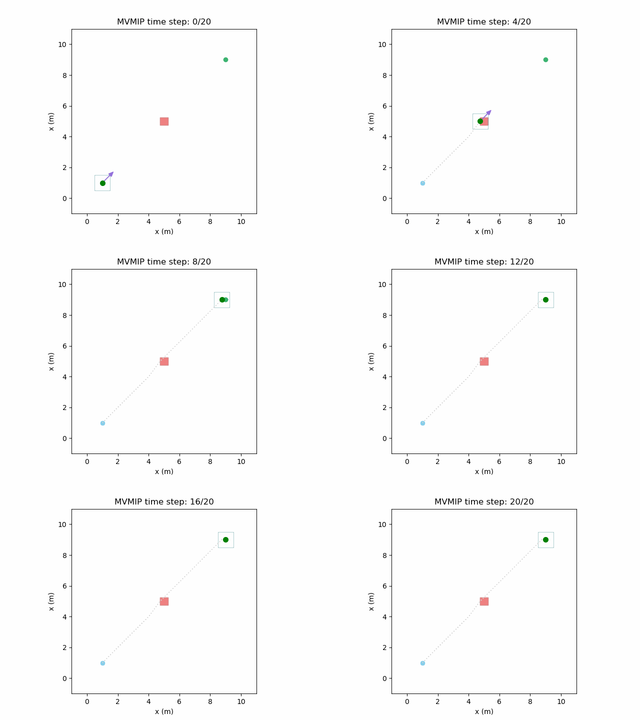
Running the MVMIP for a single vehicle and obstacle results in this:
Turns out that we’ve run into a classic problem in planning caused due to discretizing the problem. Because we only have collision constraints at each state and not in between successive states, if our control inputs have large limits, the MVMIP can find a solution that jumps through obstacles. It thinks that the trajectory is feasible because each state alone is collision free, but the reality is that the robot can pass through obstacles between discrete states.
How do we solve this? The simple LP formulation of the MVMIP makes it rather difficult to express anything too complex. We could model the space between successive states as another convex polygon and set up approximate constraints. An easier and less expensive way would be to just reduce the bounds of the control inputs such that each control step is guaranteed to move the robot by a maximum distance that is less than the size of the smallest obstacle.
\begin{equation} \begin{aligned} u_{p, max} = \max_{u}\delta_{max} \approx \max_{u}u\\ \text{s.t.} \ \ f(s, u)\Delta t \le \max{(\xlmax - \xlmin, \ylmax - \ylmin)} \end{aligned} \end{equation}
This obvious has its own downsides of limiting the max control input that can be applied, among others limitations, but keeps it simple in the spirit of the algorithm.
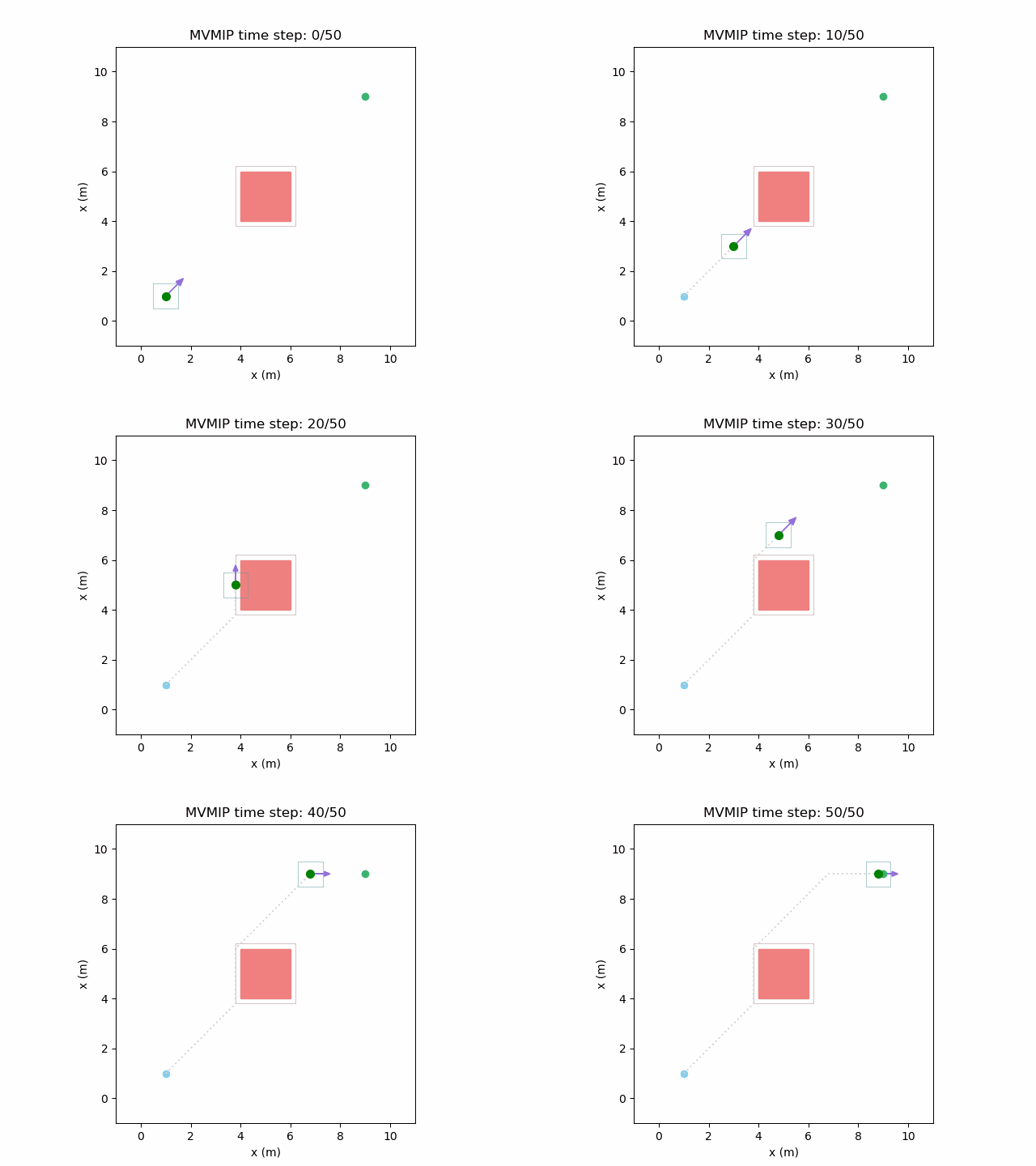
Fixing the control limits now gives us the solution that we need:
We can see that the vehicle maintains clearances to the obstacle as required, as is visually seen in the drawn boundary around the obstacle. The boundary around the vehicle itself is for vehicle-vehicle clearance.
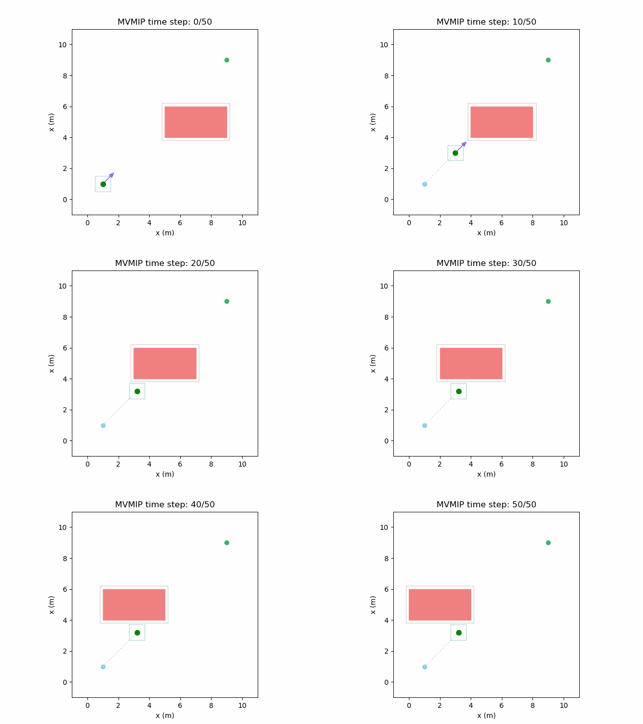
We can verify that it works as expected even with moving obstacles:
Now we can start messing around with some of the costs. To break it down, we have the $q$ vector costs on the state, $r$ vector costs on the control and $p$ vector costs on the final state. The $q$ costs encourage the robot to make progress towards the final state $s_f$. The $r$ costs encourage the robot to minimize the total control effort exerted and the $p$ costs encourage the robot to reach the goal by any means necessary.
By changing their relative magnitudes, we can achieve a range of behavior and decision making. If $q$ and $p$ are kept low and $r$ is high, the robot has no real incentive to move at all as it can minimize its total cost by staying in place. Any movement would accrue a large cost due to the high $r$ term which would overpower any reduction in $q$ or $p$ costs due to moving closer to the final state.
Making $q$ and $p$ moderately high while keeping a high value of $r$ can make the robot make progress towards the final state but stop when it has to make too much of a detour as that gets translated to applying higher control effort on average due to the longer path it will need to take. This can be seen here:
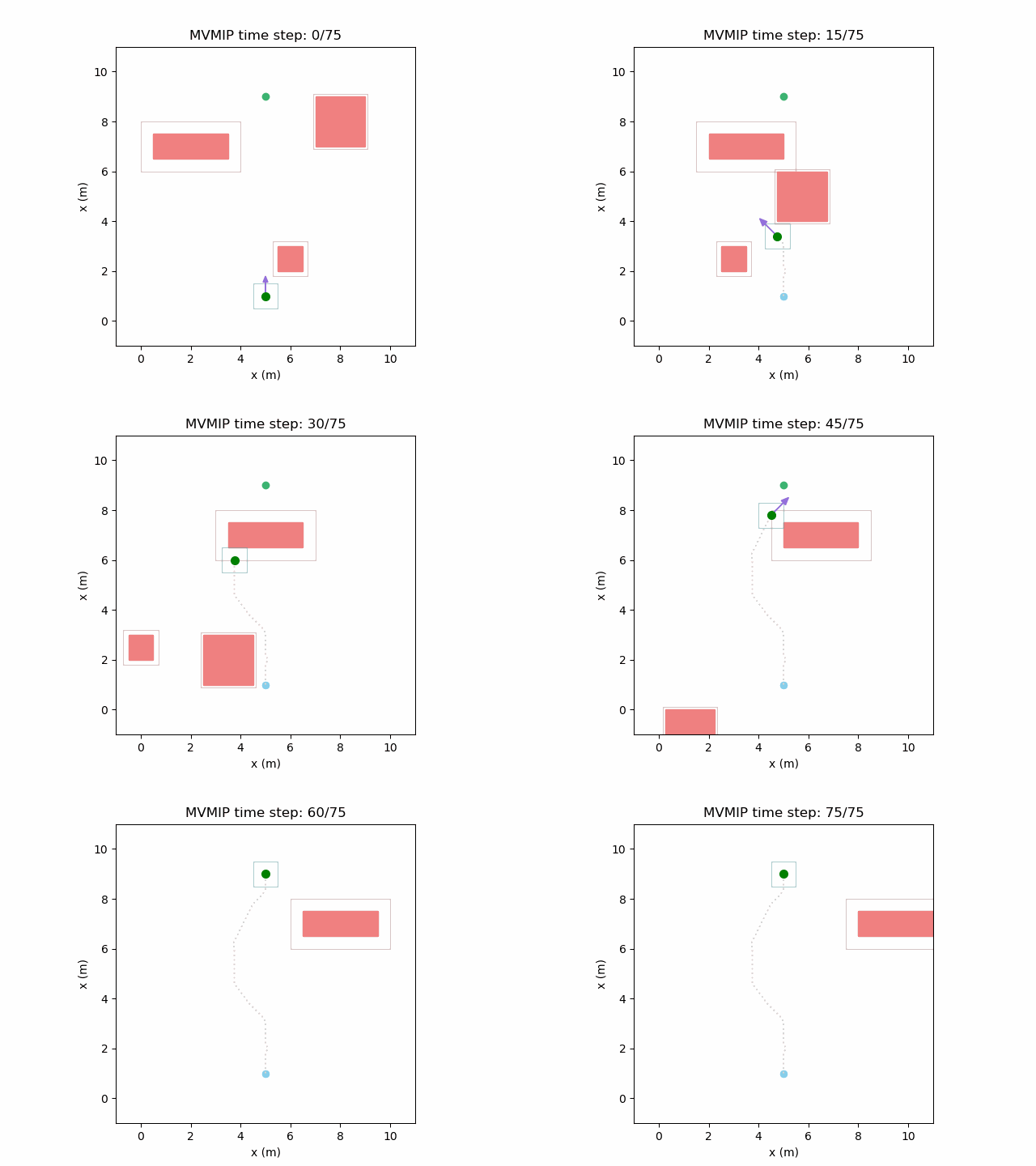
We can further see the effects of different costs on this environment with multiple moving obstacles. High $q$ and $p$, along with low $r$ will manifest in the form of aggressive decision making as expected.
Reducing $q$ and increasing $r$ can make it act more conservatively.
And finally reducing $q$ and increasing $r$ further can make it extremely passive. In this case it patiently waits for each obstacle before making its way forward. Note that $p$ needs to be very high in this case to reward it for making it to the final state. Otherwise, it will refuse to move at all.
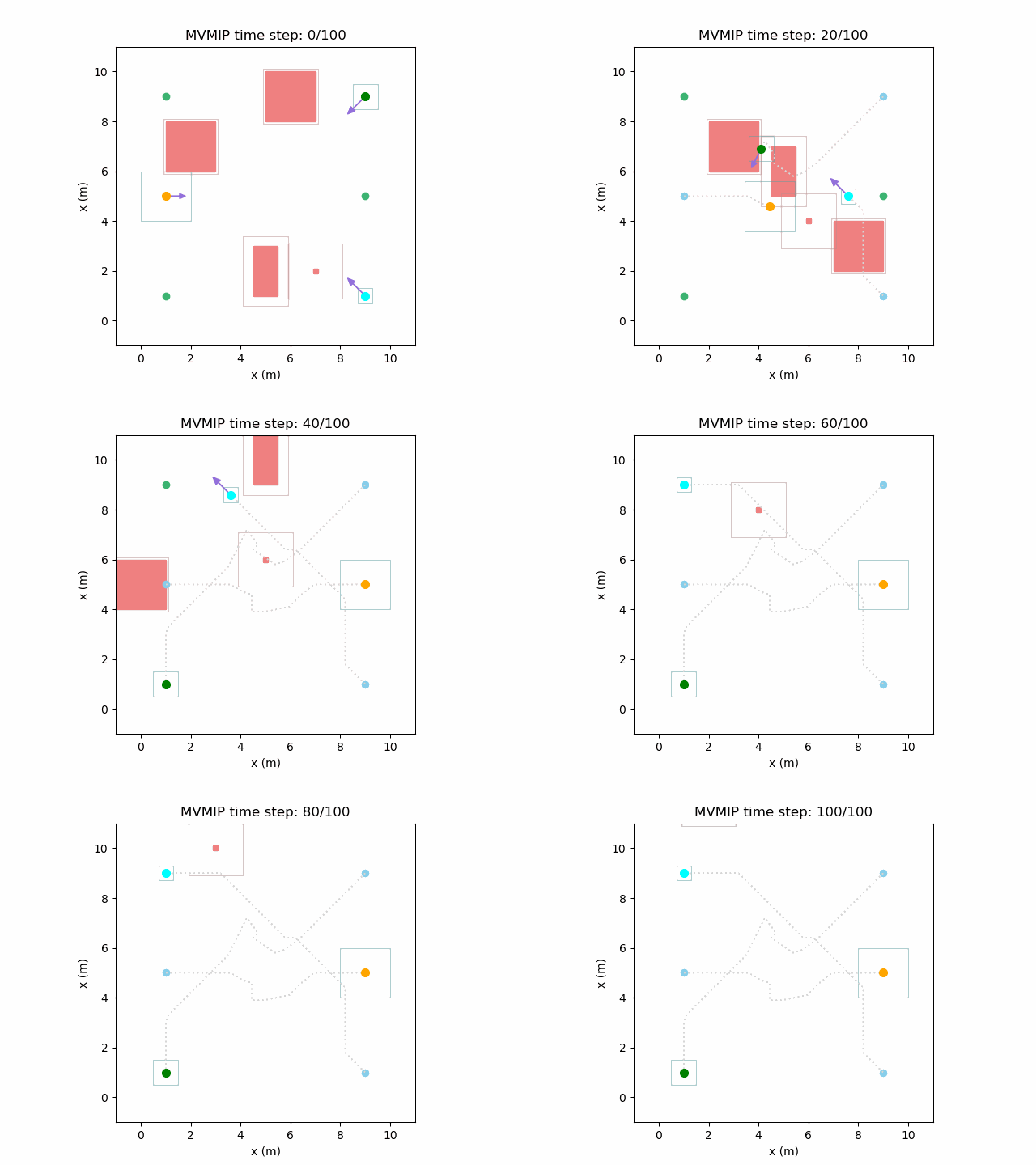
And finally, we have an example of the MVMIP in all of its glory – multiple vehicles along with multiple obstacles.
Each of the vehicles here have different costs and we can clearly see that they each have a different level of aggressiveness in their decision making.
Computational Cost
How expensive is it to solve the MVMIP?
For small problems (Like the first one shown here), it can be pretty quick.
The single vehicle, single static obstacle case had 240 variables and 300 constraints and was able to be solved in around 10 ms.
The last one – multi vehicle, multi dynamic obstacle case had 8400 variables and 10500 constraints and took upwards of 30 min to solve. Obviously there are other factors such as how easy it is to actually find a solution given the constraints and so on, but in general the solve times explode as we have more vehicles and obstacles.
Some of this can be mitigated by using the receding horizon approach.
References
- Schouwenaars, T., De Moor, B., Feron, E., & How, J. (2001, September). Mixed integer programming for multi-vehicle path planning. In 2001 European control conference (ECC) (pp. 2603-2608). IEEE. [Link]
- Richards, A., & How, J. P. (2002, May). Aircraft trajectory planning with collision avoidance using mixed integer linear programming. In Proceedings of the 2002 American Control Conference (IEEE Cat. No. CH37301) (Vol. 3, pp. 1936-1941). IEEE. [Link]
