Setting Up a Robotic Manipulator -

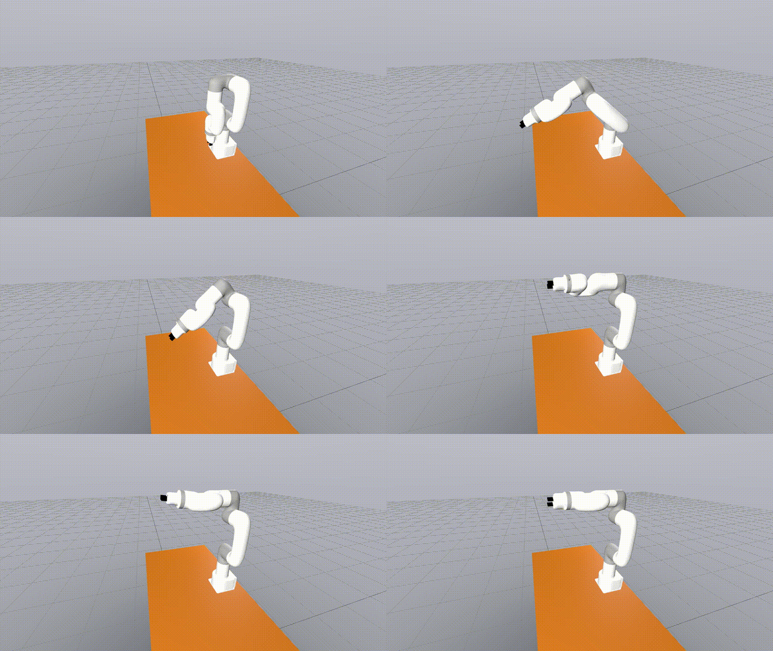
Let’s take a look at how we can set up a framework for streamlined simulation and hardware control of a manipulator. The robot under consideration is Ufactory’s Lite6 manipulator and the simulation/setup tool used is Drake.

All the code used in this post can be found in my repo. But before we start, some explanations are in order.

Lite6?

The Lite6 is one of the more economical (not to be confused with cheap) manipulators one can buy, especially for personal research where you’re not going to be spending tens of thousands of dollars on some of the more well established robots out there. It’s well built, has surprisingly good specifications for the price point, and comes with an integrated controller. You can get a parallel and vacuum gripper for it, but also comes with hardware interfaces that can support custom grippers. The product is well supported and their API (python and C++) is easy to use. The main pain point is its parallel gripper, which can only open by 1.6 cm. This severely limits the type of objects you can pick/place, but luckily for us, pick and place is only a small part of robotic manipulation!

But overall, it’s a pretty polished product that would serve well for any semi-serious research endeavours.

Drake?

In a world were robotic simulation recommendations are usually one of MuJoCo, Gazebo, PyBullet or IsaacSim, Drake $[1]$ is an extremely underrated piece of software. I’ve used it a bit previously but coming back to it after 4 years or so has been a pleasant surprise. If you’re looking for reasons for using it, here are a few:

It is still under active development and continues to mature as a robotics toolbox
Their contact models have evolved over the years and you have more flexibility in choosing the right model and simulation framework for your specific task (More on this later)
It isn’t just a simulation engine. It can do dynamical system design, control, planning and numerical optimization. It comes with out of the box implementations of common robotics algorithms and utilities
It comes with support for message passing using LCM, which is based on the UDP communication protocol. This enables Drake to be used as a replacement for ROS
It also has support for sensor and camera integration. There is also a (relatively) new wrapper around Gymnasium for more RL oriented research
Drake’s python bindings have grown over the years and is at the point where most of the library can be accessed through python

All in all, Drake gives you a lot for its generous BSD-3 license. To me, it’s become a no-brainer for any model-based robotics project.

Robot Model

The first order of business is to get the robot’s description files. Description files are used to represent the physical, kinematic and dynamic properties of a robot, usually in an XML format. The most popular formats these days are URDF, SDF and MJCF.

Ufactory provides a URDF xacro for the Lite6, which can be found here. I don’t enjoy dealing with xacros in general, as it forces you to use the ROS ecosystem. At the very least, it forces you to spend time on compiling everything and producing URDFs.

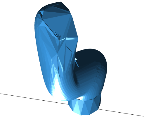
The model provided by them has a few problems as well. The collision meshes provided aren’t particularly good. For collisions, you typically want low poly conservative approximations of the actual meshes. But some of their geometries aren’t really clean. Here’s exhibit A:

But the primary problem, is the model of the parallel gripper. The actual hardware has a parallel gripper actuated by a linear actuator. It’s also open loop, in the sense that you cannot control the actual positions of the prismatic joint. The gripper can be open or closed and nothing else in between. This poses a problem in software, but we’ll get to that later. For now, the problem is in the description file. The URDF of the robot (after compiling it from the xacro), does not have actuated parallel grippers. It doesn’t even have the parallel gripper links, which is what we would need to simulate any kind of manipulation task.

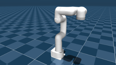
The only other model of the robot that I could find (at least at the time of writing this) is this MJCF from DeepMind’s MuJoCo Menagerie. Unfortunately, this one doesn’t have a gripper either, and utilizes the same collision meshes. Here’s a screenshot from their GitHub page:

So, we have our work cut out for us. We’ll need to make a few changes to the model, before we can actually use it for anything useful. This is usually going to be the case with most robot description files, as you’ll need to make changes to suit your particular application.

Collision Meshes

Most simulators don’t support collision checks for non-convex meshes/geometries as this is more challenging to compute and is more expensive than doing it for convex shapes. Given non-convex meshes, most simulators will either try to approximate the mesh by a set of convex meshes, or compute a convex hull of the mesh. Ideally, we’d like to control the behavior, instead of letting the simulator decide something internally.

For our case, we can take one of two approaches:

Manually compute a low poly representation of each link as a collection of low poly convex meshes
Represent each link as a collection of basic geometries (cuboids, cylinders, ellipsoids, etc.)

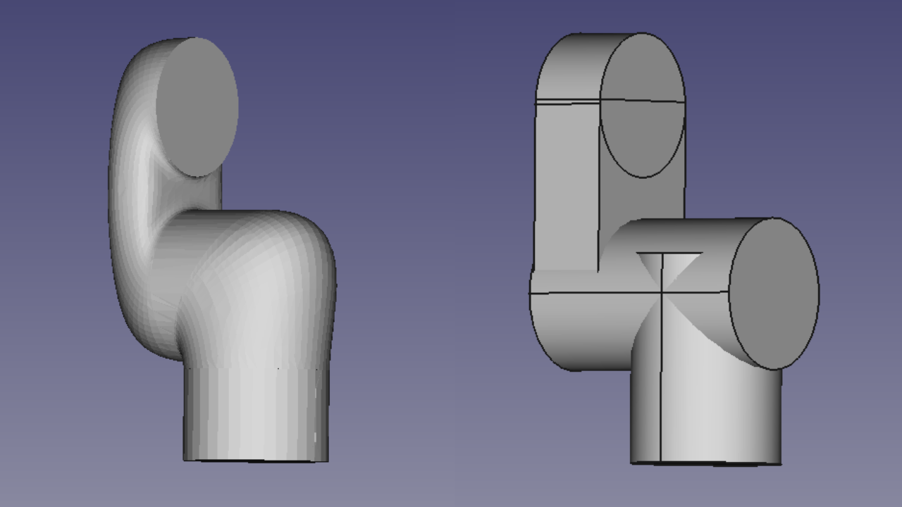
The second option is the more computationally tractable one and makes it so that you don’t have to deal with the original meshes at all (other than using them as a reference). It has the disadvantage of being more conservative and increasing the likelihood of spurious collisions, but we can be a bit smart about how we build these geometries by not incorporating parts of the meshes that are extremely unlikely to collide with anything.

Here’s an example of what this process looks like for a particular link on the robot.

Parallel Gripper Model

To model the gripper, we do the following:

Add the two parallel gripper links according to the dimensions of the actual gripper. The actual prongs of the gripper are rectangular, which makes it easy to specify the visual and collision geometries
Add joints to specify the max and min gripper movement, along with actuators to enable simulation. We also make sure to set the effort and velocity limits (taken from empirical measurement using the real hardware) and specify inertial properties as well. The mass in this case will need to be approximated as there’s no real way of measuring this without taking the gripper apart

We could model this using a single actuator, with a URDF mimic joint on the other actuator, but Drake doesn’t play nicely with this setup. So we use two actuators and deal with any complications through software.

The gripper can also be installed in two ways: normal and reverse. The normal configuration has the gripper width go from 0 to 1.6 cm, while the reverse setup as it go from 2.2 cm to 3.8 cm. As mentioned before, the gripper specs are very limiting, but we try to make the best approximation of the actual hardware.

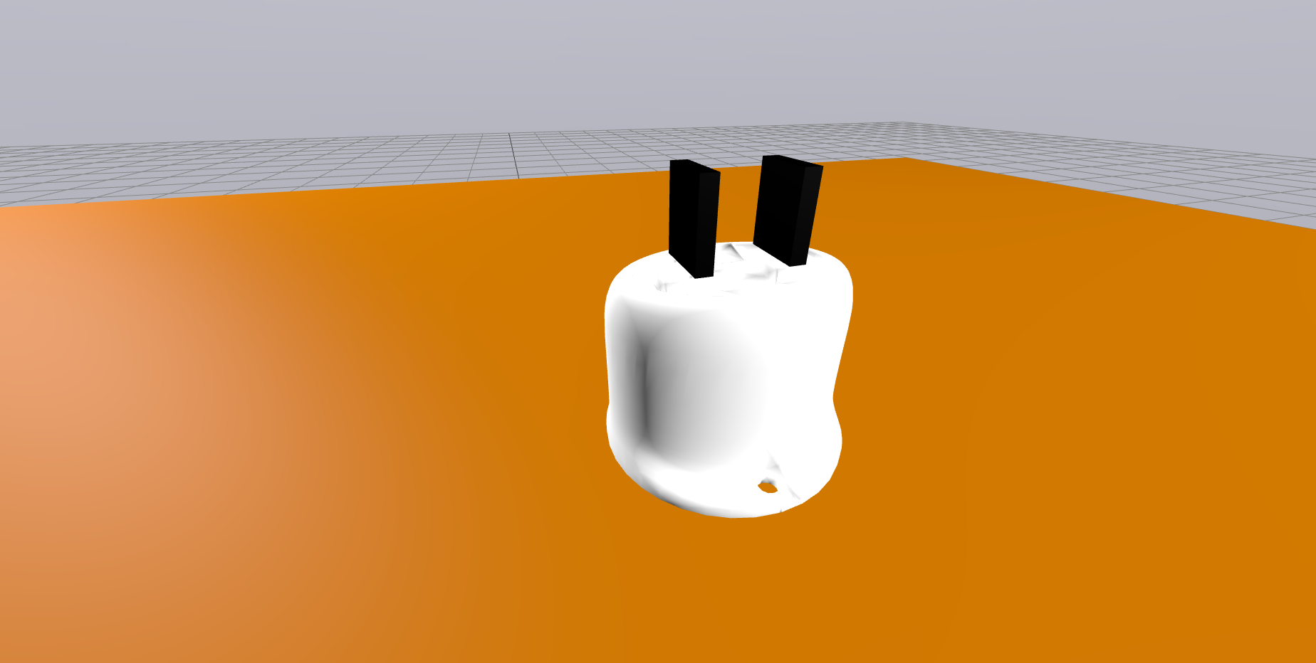
After modelling, this is what the gripper’s reverse configuration looks like:

Inspection

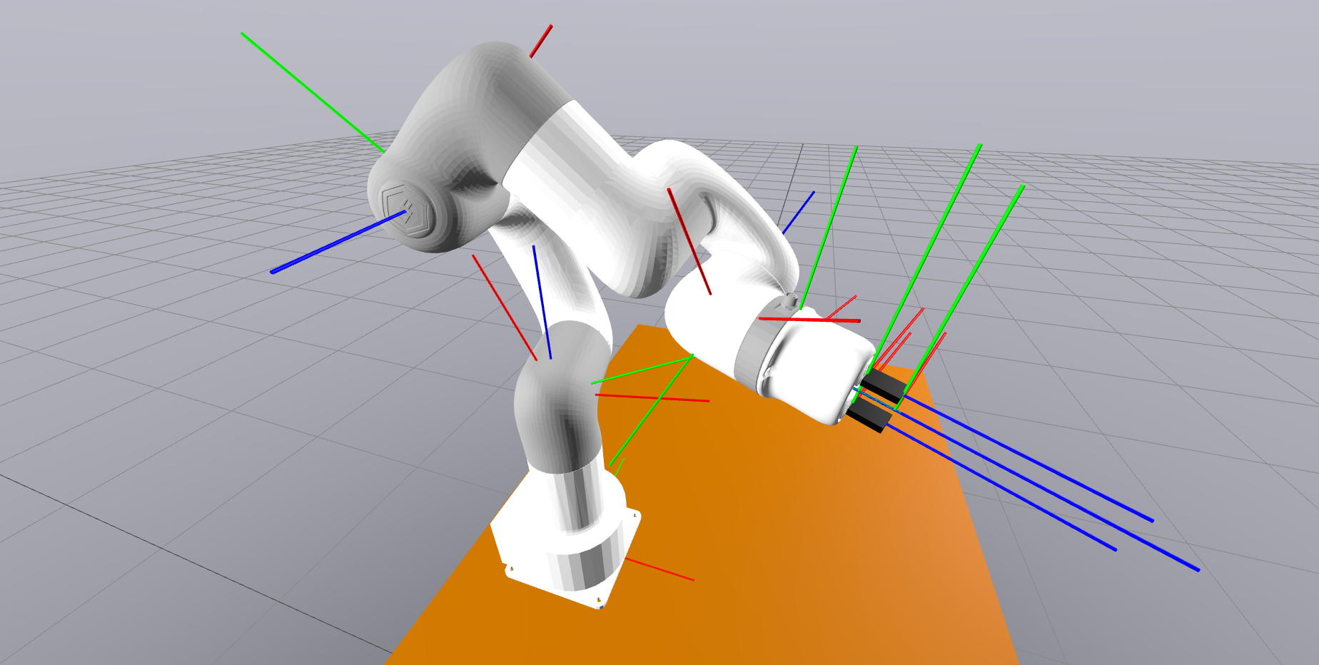
We can now put everything together, visualize the robot in Drake, and run some final inspections. The first thing we check is that the each link’s coordinate frame is placed and oriented correctly.

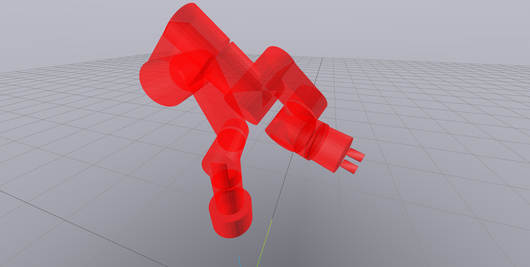
Next, we check what our custom collision meshes look like.

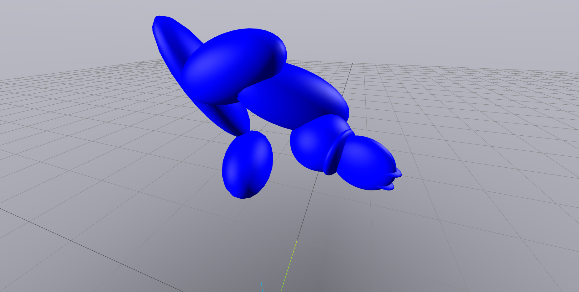
We can see how the basic geometries make up for a clean approximation of the original meshes. Finally, Drake also allows us to visualize the inertia tensors of each link as an ellipsoid. This can help us verify that the inertial parameters provided in the original description by the manufacturer is in fact correct.

It’s easy to get these values wrong, and is equally difficult to actually fix them if they’re incorrect. But in this case, they seem to be accurate. Lucky!

Drake Specific Setup

Finally, we need to add certain Drake specific information to the URDF file. Drake extends the description file format to include additional tags that it can use to better model the dynamics of robots. Details regarding this can be accessed here

We add the drake:declare_convex tag to each collision geometry mesh. This tells Drake that it can assume the mesh to be convex and not have to do any convex hull computations
For URDFs, Drake doesn’t parse the mechanicalReduction tags of an actuator. Instead, to specify the gear ratio, we add the drake:gear_ratio tag
For motors with a large gear ratio, the inertia of the rotors can significantly affect the dynamics of the system. If these values are known, they can be added using drake:rotor_inertia. Unfortunately, these are not known for the Lite6 manipulator, so I’ve not included them in any of the models
To enable hydroelastic contact, we need to add drake:proximity_properties to each model/link that can make contact. More on this in the pick and place section

We now have a description model that can be used for all sorts of simulations. My version of the models with compiled URDFs can be found here. I have models for each of the following setups:

Manipulator without gripper
Manipulator with normal parallel gripper
Manipulator with reverse parallel gripper
Manipulator with vacuum gripper
Separate normal parallel gripper model (without the rest of robot)
Separate reverse parallel gripper model (without the rest of robot)

There are also separate models for Drake and non-Drake use. Each model includes the simplified collision geometry meshes, along with OpenCAD files containing the CAD source for the simplified collision geometry.

Simulation And Hardware Setup

Almost everything in Drake works around a Systems framework, where individual systems are modelled to take in certain inputs through input ports and output its results through output ports. This setup enables us to not just simulate our robot, but also build an integrated system that can both simulate and be run on real hardware. By building such a system and swapping out some of the components inside it depending on whether we want to run our algorithm in simulation or on the actual robot, we can build a framework that allows for quick prototyping and development. We can test something in simulation and by a flip of a switch (or flipping a boolean/Enum in software terms), we can run the exact same code on real hardware and have the simulated behavior be accurately transferred. The idea is inspired from Dr Russ Tedrake’s manipulation repo, that he uses for his Robotic Manipulation course at MIT.

How exactly do we achieve this? We start by building a Drake Diagram that is a collection of different individual systems. I call this system a MultibodyPliant (Henceforth referred to simply as pliant: A play on Drake’s MultibodyPlant. Pliant because of its flexibility in being able to be used for both simulation and hardware!). Disclaimer: The rest of the post will use some Drake jargon. I’ll defer their explanations to Drake’s documentation.

Basics

We first set up the Diagram to enable simulations. Before we start, we need to know how the Lite6 API functions and what it lets us do. This is important because we want to model the simulation to take in the same desired inputs and work the same way as the controller on the robot. Looking at their API (python and C++), we can see that it supports both position and velocity control of the joints. It also supports cartesian end effector control, but this is not something we’re going to be using as the aim is to write algorithms that will do so.

I’ve implemented both position and velocity control in my repo, but I’ve only thoroughly tested the velocity control aspect of it. The rest of the post will only consider the velocity control scheme. We also only deal with the parallel gripper for the time being.

So here’s what we need the simulation system to do:

Take in desired joint velocities (as a vector of 6) as input
Take in a desired gripper status and actuate the gripper based on this status.

There is some complexity with the second point. Having actuated grippers in the model means that Drake’s representation of the model has 8 joints and velocities (2 additional DOF for the parallel gripper) for a total of 16 states instead of the 12 on the actual robot. On the real hardware, the state of the gripper isn’t fully controllable – only as an on/off switch, so we need to simulate this behavior as well.

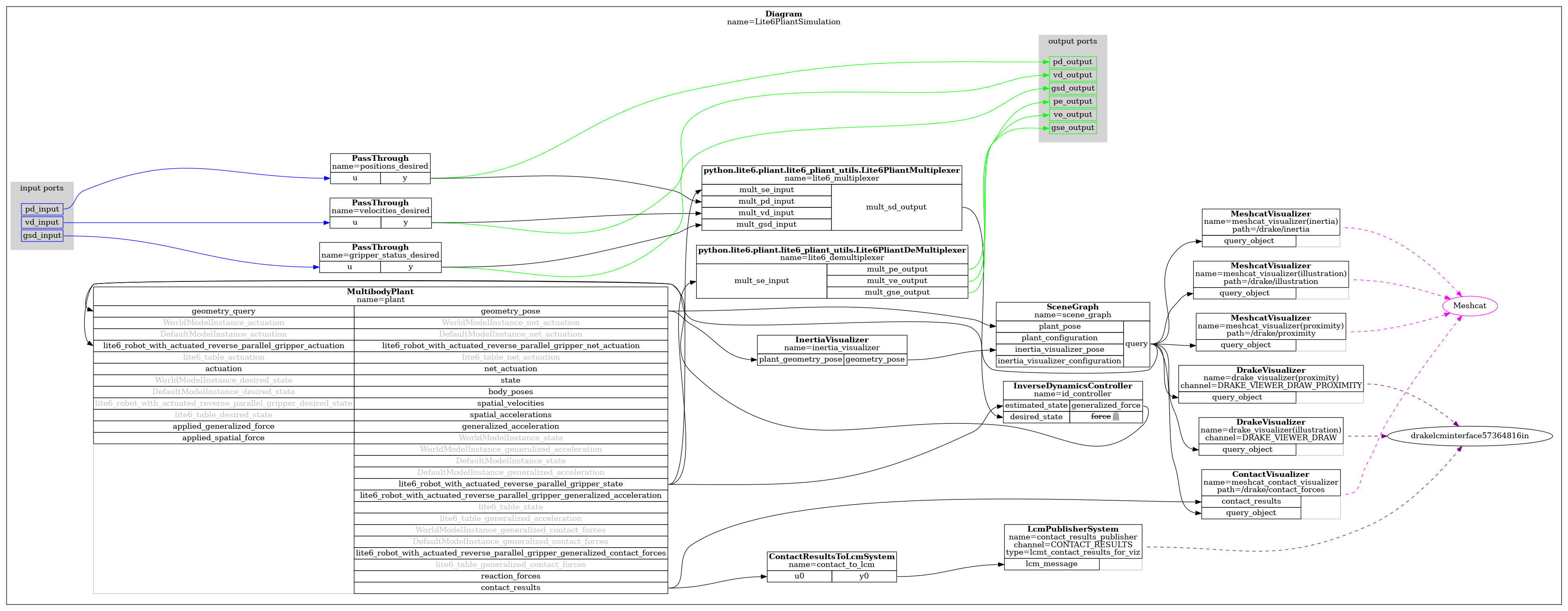
Drake lets you generate a pydot representation of any system you build. This is what the entire pliant looks like:

(What is this? A diagram for ants? Please do zoom in) It might seem overly complicated, but a lot of it is just fluff, I promise!

The system takes in the desired positions, velocities and gripper status as inputs. We don’t require positions for velocity control, but we do for position control, both of which are implemented using the same pliant.
The input desired positions and velocities are each size 6 vectors (corresponding to each joint) and the gripper status is an Enum that can be OPEN, CLOSED or NEUTRAL. To get this into a Drake system, it is wrapped into an AbstractValue and sent through an abstract port.
These desired velocity values are also exposed as output ports of the pliant

Modelling The Hardware Controller

For the actual physics simulation, we embed a MultibodyPlant of the robot model into the system. Most simulators require force inputs (torques for the joints in this case) in order to step forward in time. So we need a system that takes in the desired velocities and computes torques that can be fed into this simulation plant. This is also the part that models the motor controller behavior of the actual hardware.

Luckily, Drake provides an InverseDynamicsController, which is a PID controller mapping from the joint positions and velocities to output torques. Tuning this PID is akin to changing the simulated model of the hardware motor controller. To do velocity control, we can set the input desired positions to the current estimated positions. The kp * (q - q_desired) term cancels out and we end up with a pure velocity inverse dynamics controller.

There is one other problem. Even though the parallel gripper gives no feedback and its positions are exactly controllable, it still has certain dynamics that the simulation needs to capture. For example, after measuring, I’ve estimated that the gripper takes ~250-300 ms to completely open/close from the opposite position. We can simulate this behavior by incorporating the gripper states, setting a desired velocity that we require and tuning the inverse dynamics PID gains for it. So we need our controller to include the gripper state (position and velocity) as well to model this, but our inputs are only 6 dimensional, along with an Enum for the gripper state.

State Management

We need to augment the input joint states to include the gripper state. This is exactly what the custom multiplexer unit seen in the graph diagram does. It takes the native inputs to the pliant and adds the gripper positions and velocities by consuming the gripper status. We have fixed values of gripper positions and velocities for each of the OPEN, CLOSED and NEUTRAL states (from measurement, product specifications and collected data). We can now feed this into the inverse dynamics controller system and have full control over the joints and the gripper.

As seen in the diagram, the output of the controller goes into the MultibodyPlant actuation input (as torques). This now enables us to simulate the robot by sending it desired velocity commands.

Finally, we want to also be able to report estimated joint positions and velocities, similar to the robot’s API. To do this, we use a custom demultiplexer unit that can go from position and velocity estimates of size 8 coming from the simulation plant into position and velocity estimates of size 6 (just the joints) and a gripper status Enum. This brings us back to our original input format, and is also the format we’ll be using for the robot hardware API calls. From the diagram, we can see the output of the demultiplexer (containing estimated states) be exported into output ports of the system.

Hardware Pliant

The last thing is to now set it up so that when we want to create a hardware pliant, it returns a Diagram that has the same input and output ports, but this time without the simulation part inside it. This is what it looks like:

This one is a lot simpler. We have the same input ports of the desired positions, velocities and gripper status, but this time instead of going into the multiplexer, it is fed into a Lite6HardwareInterface block. This system embeds calls to the robot hardware API inside it. Every step, it commands velocities to the robot, and also updates its estimate of the joint positions and velocities. This estimate is sent through to the output ports.

The only difference between the hardware and simulation pliants are what the inputs command and where it gets its state estimates from. For simulation, it computes the commands through the inverse dynamics controller and sends it to the Drake’s simulation plant. The simulation plant also provides estimates of the state by stepping the simulation forward in time, which are then exported as outputs. For hardware, the desired velocities are directly sent to the robot and estimated state is directly read and exported.

Something that I ran into is the problem of specifying updates for the hardware system. Unlike the simulation pliant, we don’t embed a MultibodyPlant object as a part of the hardware pliant, and stepping the simulation forward will cause it to skip all the way to the end as there are no defined update events. But the goal is to be able to run the same program on both simulation and hardware without having to make any changes. So this means that we need to create update events for the system at some control frequency that we wish. I’ve tried a bunch of things here (like having separate publish events, etc), but what I ended up liking the most and going with is:

Declaring a DiscreteState containing the last updated values of the estimated positions and velocities.
Declaring a periodic discrete update event at a chosen frequency. This event will both send the current commands (desired joint velocities) and update the latest state estimate every update step.
In the future, we could also have two events – one for commanding and one for reading the state estimates. This will enable us to send commands and update state estimates at different frequencies

Something else to keep in mind is that, if we declare the outputs ports for the Lite6HardwareInterface with the setup described above, it will lead to an algebraic loop when used as a part of actually running a simulation, which Drake does not support. This is because the by default, the output of the system is considered to be a function of its desired state inputs (not true as it purely comes from the robot API calls). This output will at some point get passed into a control/planning algorithm, the output of which will connect back to the desired state input. To avoid this, we need to make sure to set the correct DependencyTicket for each declared output port of the hardware pliant. In this case, declaring that the outputs only depend on the discrete state will get everything to play nicely with each other.

And that’s it! We now have a system that can be used to both simulate something, or run it on hardware, by only changing a single flag.

Analysis

Before we can put this system of ours to good use, we want to check the accuracy of the simulation. If the simulation isn’t good enough, it defeats the idea of a having single system for simulation and hardware control.

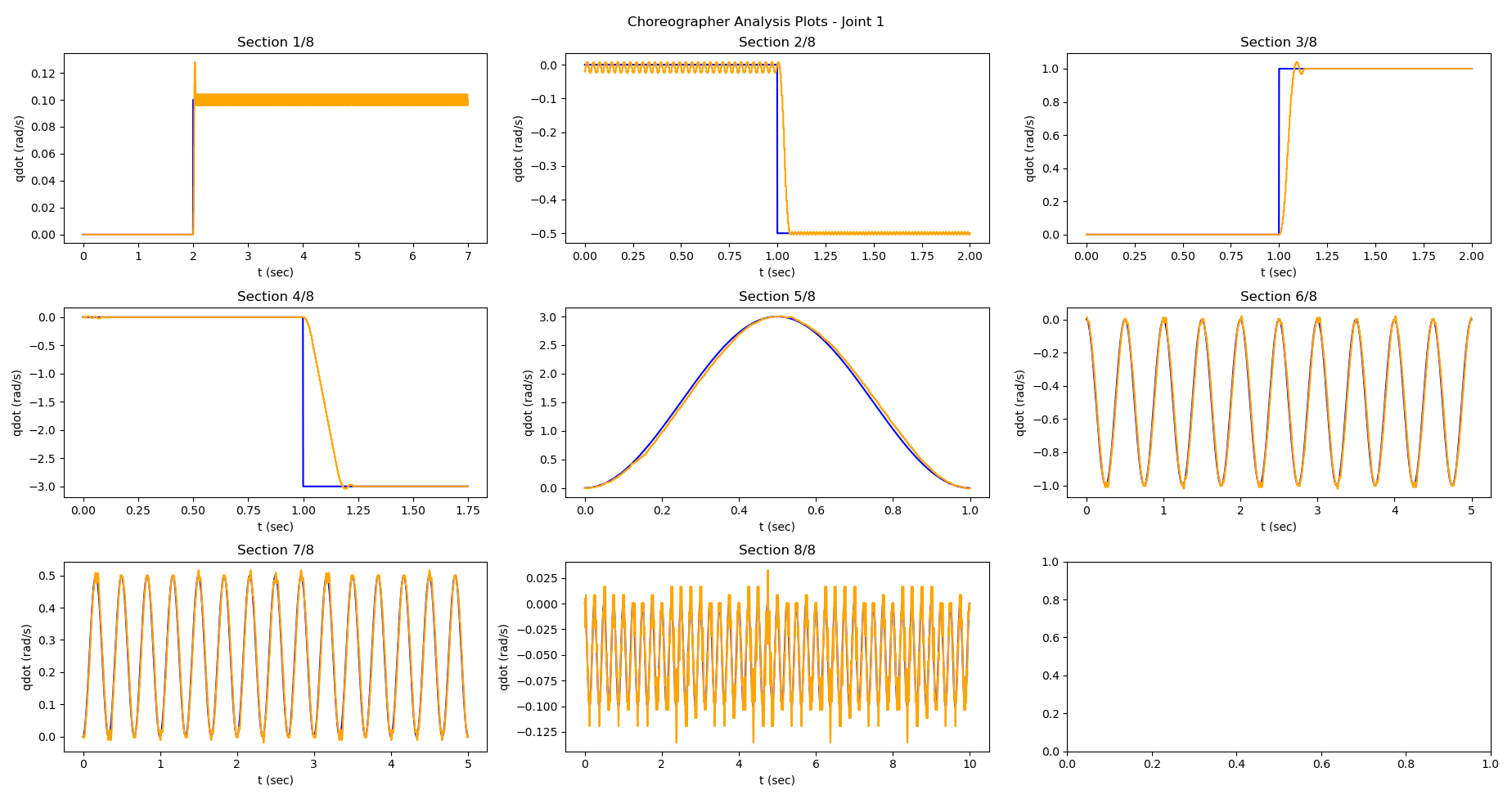
To do this, I built a Choreographer system that sends specific velocities to each joint at a time and measures the response of the robot to the inputs. To keep it simple, the input velocities are all step and sinusoidal signals. The code for this part can be found in the analysis directory of my repo.

Here’s what the entire sequence looks like in simulation (run in real-time). It’s 12 minutes long, so I wouldn’t recommend watching the entire thing.

For each joint, we test for both low and high velocity responses. The max velocity for each joint is +/- 3.14 rad/s, so we test the responses for discrete velocities between 0.1 and 0.3 rad/s which will cover most of the working range. It is also executed for different arm configurations (folded in, stretched out, etc.) to check the response for different load conditions.

We first plot what the desired and response velocities are for the actual hardware. This is what the plots look like for the first joint:

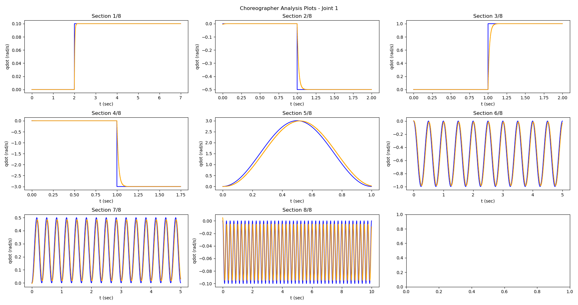
We can now plot the same responses for the simulation and then do a bit of inverse dynamics PID tuning to get the response we need.

It looks pretty good, but suffers a bit at higher velocities. We can see that the actual dynamics at higher velocities tend to be more sluggish. The problem with the velocity control setup currently is that the kp gains don’t do anything as we set our desired and estimated positions of the inverse dynamics controller to be the same to achieve pure velocity control. So the PID tends to be just proportional control on the derivative terms (velocities). This explains the graphs we see, as they correspond to high kp gain responses. To get closer to the hardware responses, something we can do is:

Decrease the kd gains (which are effectively the kp gains for the velocities) for the joints to make the responses more delayed at higher velocities
Set up a discrete derivate block and compute a manual kd* term after taking a derivate of the target and estimated velocity difference (accelerations). This can then make up for the responses not hitting the target velocities at the lower end fast enough due to reducing the proportional gain

But for now, we can just stick with the current model, as it pretty accurately describes the responses at lower velocities. Most of our applications are going to be within this range, and we will seldom need to go whizzing at 3 rad/s.

Simple Pick And Place Application

We’ve gone through the gruelling task of fixing the description files, setting up utility code and analyzing what we have. We’re finally ready to put our system to good use.

To demonstrate the capabilities of this setup, I built a gripper pose tracking controller for a simple pick and place setup. There is no vision in the loop, and we assume that the positions of all the cubes in the setup are known by the robot.

For the controller, Drake’s DoDifferentialInverseKinematics comes in handy as it lets us go from end effector to joint velocities. The geometric Jacobian required by the function can easily be obtained from the MultibodyPlant, but there is a problem here. Our robot model requires 8 positions and states, so going into and out of this controller will require more multiplexing and demultiplexing. It’ll also require us to cut off the gripper parts of the Jacobian. Instead of going through all of this, another option is to have separate robot models with non-actuated grippers (The parallel links still exist, but are not actuated. They are connected to the gripper base through fixed joints).

This being a simulation involving contact, there is something else we need to consider. Running it the way it is will result in Drake using its point contact model. This is fine, but we can do better.

Simulators in general don’t like surface to surface contact as it can result in discontinuous and non-consistent forces when they try to model them as point contacts. A popular way of dealing with this is to modify the collision geometry itself by shrinking the collision meshes a bit and adding spheres of very small radii (The order of 1e-6 m or lesser) at relevant points. So for a cube, the collision geometry will be a cube that’s slightly smaller, along with 8 spheres at the corners of the cube. By doing this, the contact points are well defined when the block is placed on a table or when a manipulator is picking it up, and can lead to more stable simulations.

This indeed works better for our pick and place example, but we can do better still. Drake’s latest and greatest contact model, called hydroelastic contact, is a surface (still compliant) contact model that takes into account contact patches between bodies. It is able to resolve contact forces within these patches and provide a richer representation compared to using a finite set of contact points. Their hydroelastic contact user guide is a very good read.

How do we enable this for our simulation? By default, drake tries to use hydroelastic contact, but falls back to a point contact model if the meshes don’t support hydroelastic contact. To enable this, we need to add the drake:proximity_properties tag to the collision geometries under consideration. Their user guide and tags page explains what each property does. But in brief:

Each collision geometry needs to be defined as a drake:compliant_hydroelastic or a drake:rigid_hydroelastic type to enable hydroelastic contact
The other important property is drake:hydroelastic_modulus (for compliant shapes). It defines the “stiffness” of the object.
Mesh tessellation is controlled using drake:mesh_resolution_hint and defines how the collision mesh is approximated. This is more important for custom non-primitive geometry meshes
The coefficient of dynamic friction value can also be provided through drake:mu_dynamic

After updating the collision geometries of the table, cubes and the parallel gripper, we’re ready to go. We can run the pick and place simulation and try running the same program on the robot. The following is what we end up with. Perfect!

References

Russ Tedrake, & the Drake Development Team. (2019). Drake: Model-based design and verification for robotics.