Atium
Atium is a more formal collection of some of my motion planning experiments, research ideas and paper implementations. Details of the individual implementations can be found within the subdirectories of the repo.
Manipulation Research
This is a collection of manipulation algorithms for execution in simulation and a real hardware robot.
Legged Research
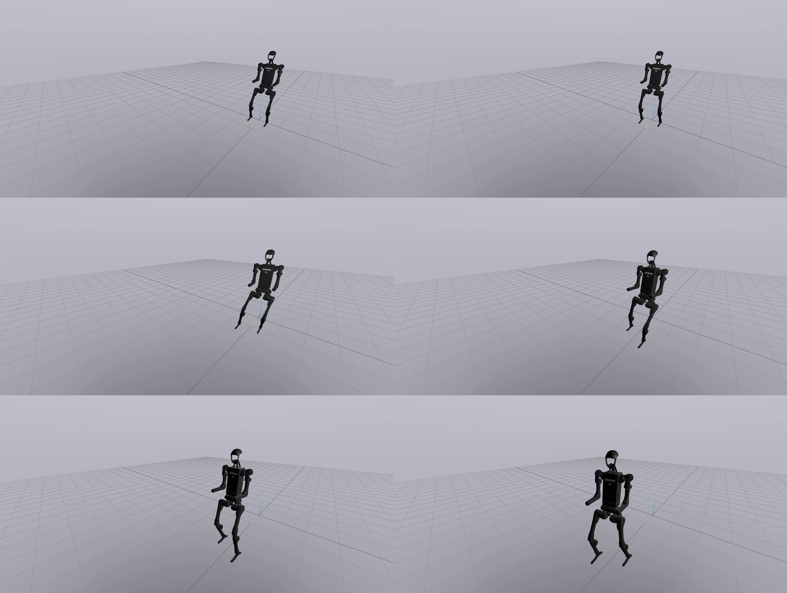
This is a collection of algorithms for legged robots. Everything here is purely simulation in Drake.
GPV
Generation of policy variations in deep reinforcement learning
The project aims to enable reinforcement learning agents to obtain probabilistically consistant policy variations from a learned deterministic policy. A Variational Autoencoder (VAE) is used to obtain these variations. The goal is to enable agents to execute actions that are different (and sub-optimal) from the trained policy, while still being able to achieve the desired result.
This is useful in cases where we need to generate behavior that is not a part of the trained policy, while also making sure that the system does not fail at the given task. It also gives the agent an opportunity to solve the task in environments that are slightly different from which the episodes were obtained.
Post-Training GPV (PT-GPV)
The post training variant of the algorithm assumes that we have an agent that has already been trained using some learning algorithm. The agent thus knows what action to take in any given state. Given such a model, a VAE is trained conditioned on the current state to reconstruct the output policy.
A VAE is used because we can control the variation in the output. By weighing the reconstruction loss of the VAE more, the variational policy is able to reconstruct the actual policy (From the trained agent) more faithfully. By weighing the the KL-Divergence loss more, we obtain a better distribution of the latent variable leading to more varying but consistent actions. This ensures that even though the actions vary depending on the sample from the normal distribution, the actions are still able to get the agent to solve the task at hand. The VAE helps obtain samples from a sub-optimal distribution around the optimal policy.
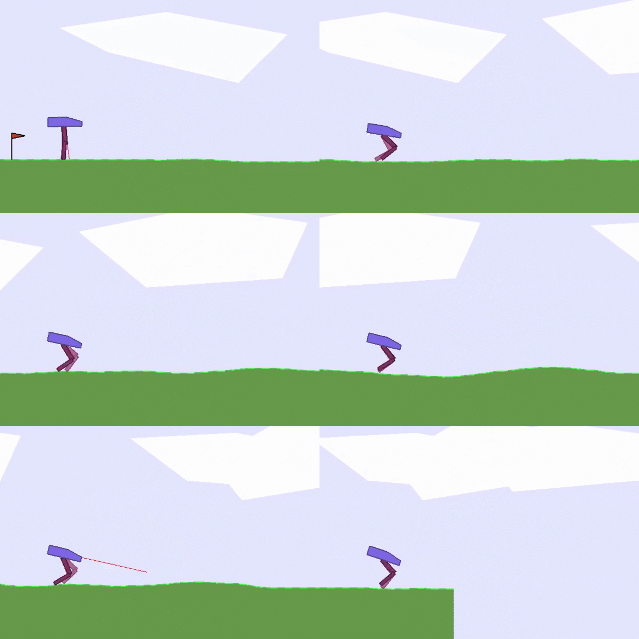
The VAE is trained using state-action pairs collected from the trained agent. The algorithm was tested on OpenAI’s gym environments. The results on the bipedal environment are shown below. On the left is a vanilla DDPG (Deep Deterministic Policy Gradients) policy, and on the right is the agent running the policy from PT-GPV.
As seen, the algorithm is able to generate behaviour not seen in the original trained model (Like jumping).
By varying the weights of the VAE losses, we can control the amount of variation in the resulting actions. As the amount of variation is increased, the probability of the agent failing to complete the task also increases.
Simultaneous-Training GPV (ST-GPV)
In this variant, the VAE is used in conjunction with a learning algorithm to help in better exploration. Finding the best exploration methods is a challenging task in policy gradient algorithms. DDPG uses predicted actions along with normal/Ornstein-Uhlenbeck noise to enable exploration. We replace this noise generation procedure with a VAE that gets trained along with the learning algorithm.
Each training iteration trains DDPG and the VAE for a set number of iterations. The training follows the structure shown below.
At first, the VAE gives more varying outputs due to not being completely trained. This leads to more exploration. As the DDPG target actor converges, the VAE output also stabilizes. The exploration decreases as the model is trained, which is the behaviour expected of a good exploration strategy. GPV can thus be used along with a learning algorithm to facilitate exploration.
Morphac
[Shelved]
Morphac (Mobile Robot Playground for Planning and Control) started out as a motion planning and control library for mobile robots. The aim was to develop a mature software library that could be bootstrapped to carry out research in areas such as planning, trajectory optimization, etc. Its backend is written completely in C++ with python bindings for actual use.
Mnyrve
[Shelved]
Mnyrve is a Reinforcement Learning library written in C++. The aim of the project is to provide implementations of useful learning algorithms as well as provide a platform to implement the more recent ones.
The library follows a module based approach, where theoretical constructs (Like value functions, policies, episodes, etc.) are written in the form of modular classes. The algorithms also follow this paradigm. This makes it easier to implement algorithms and also implement new ones.
The core library is built using C++. The Eigen library is used for all linear algebrary and matrix operations. Python is used for all visual and graphical representations. The Bazel build system is used to build the project.
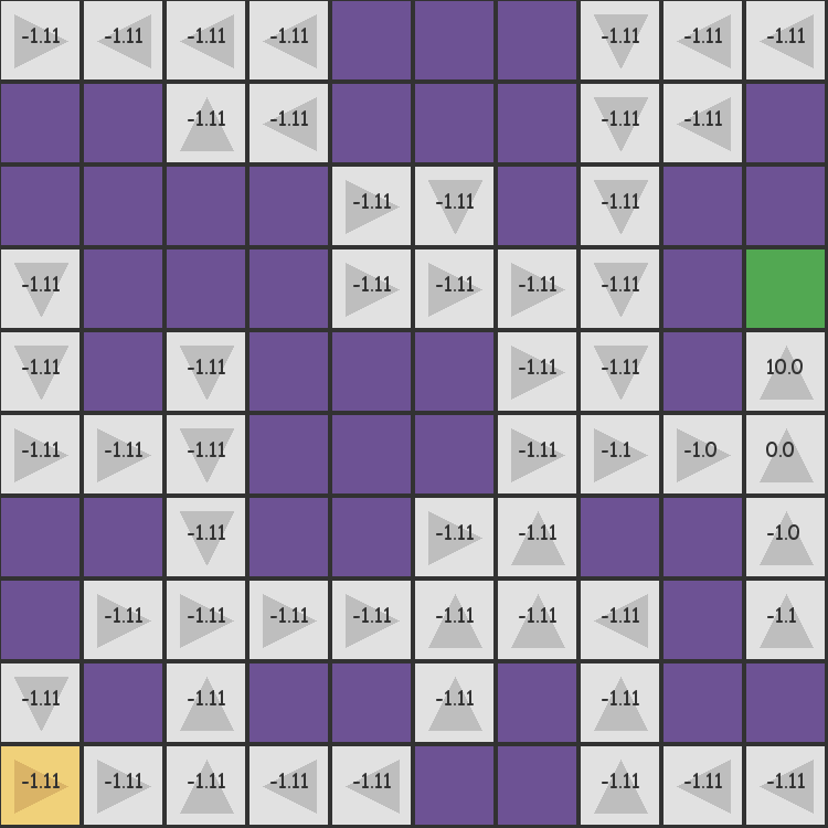
An example of the output of the value iteration algorithm on a simple gridworld is shown below.
PTE
Parametric Trajectory Estimation
PTE explores methods to use data from previous trajectory optimization solutions to enable obtaining faster optimization for further problems (On the same system). Two approaches have been explored:
- Fitting parametric curves on the trajectory data to obtain better initial seeds for new initial states.
- Reusing parts of older trajectories and minimizing the amount of new trajectory data needed to solve a problem.
For fitting curves, the idea is to compute a general curve that only depends on the starting configuration. The assumption made is that the control problem solves the same task and has the same goal state. Given all the previous trajectory data with their initial states, we fit a least error curve parameterized by the initial state of the system.
Single Polynomial Spline (SPS)
In this model, a single high degree polynomial spline is fit to the trajectory data. The fit obtained was of high error due to the inherent coupling between state transitions. Being a single spline, the knot points in a neighbourhood would all be dependent on each other and cannot be moved independently.
If the degree of the polynomial is too low, it would not be able to express the trajectory well enough. On the other hand, if it is too high, we end up with a lot of variation and lose generality. This model thus performs poorly, especially when the state space dimensions are high.
Point-wise Spine (PWS)
To deal with the issues faced by SPS, a point wise spline model is introduced. The spline models each knot point separately (parameterized by the initial state), which helps in removing unnecessary dependencies between the knot points. As each knot point parameter is now independent, failure to capture trends in a particular region in the trajectory will not affect other regions.
As expected, this model works better than SPS and gives us impressive results. The parameters of the curve are found by formulating an optimization problem. A simple squared loss ensures that the problem is convex and the best possible generalized curve is found for the given data.
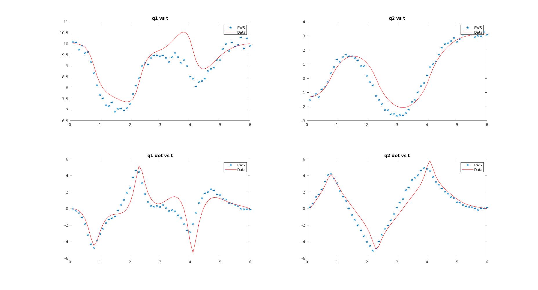
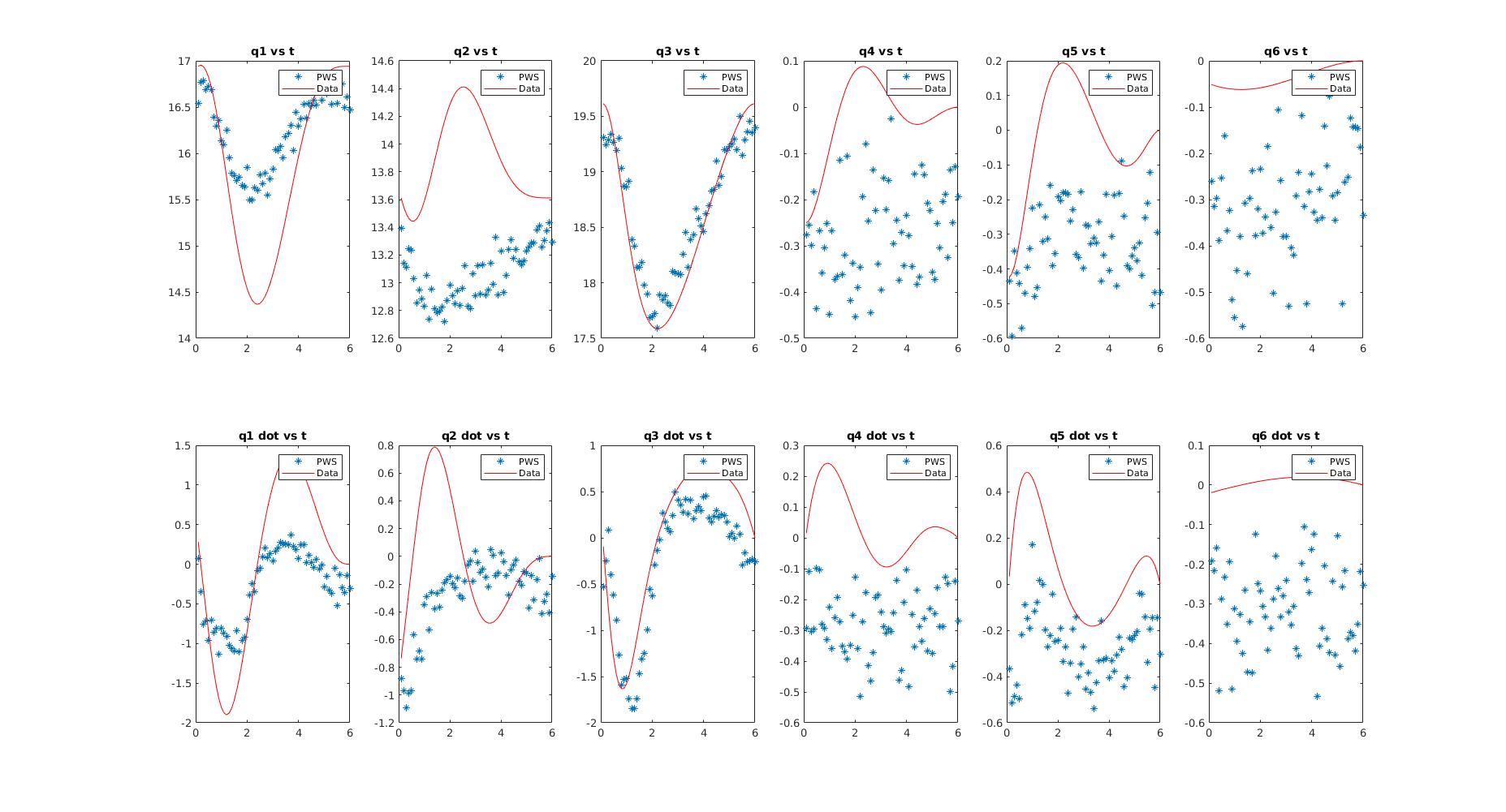
Data for the results were obtained using direct collocation on simulations of the cartpole, acrobot and quadrotor models. The following figures show the curves found after optimization for the cartpole and quadrotor states.
The least error trajectories are very accurate for lower dimensional systems (cartpole) but tend to start deviating away for higher dimensional systems (quadrotor). But even for the higher dimensional systems, the states corresponding to the positions are well tracked and give reasonably good estimates.
For new states, the predicted trajectory is then obtained by using the curve parameters. The knot points in this trajectory is then used as the initial trajectory to solve the direct collocation problem for the new state. The idea is to reduce the number of iterations required by the solver by providing better initial trajectories.
Results were tested on the cartpole and quadrotor models. The cartpole has a total of 4 states, the goal state being the upright position. The quadrotor has 12 states, the goal state being a state with zero velocities (Perfectly balanced). The following tables compare the results of optimization with and without PWS for the cartpole and quadrotor respectively.
| Cartpole Evaluation | Iterations without PWS | Iterations with PWS | Function evaluations without PWS | Function evaluations with PWS |
|---|---|---|---|---|
| 1 | 175 | 983 | 142 | 483 |
| 2 | 149 | 726 | 130 | 759 |
| 3 | 144 | 664 | 53 | 122 |
| 4 | 211 | 957 | 81 | 256 |
| 5 | 196 | 1064 | 53 | 111 |
| Quadrotor Evaluation | Iterations without PWS | Iterations with PWS | Function evaluations without PWS | Function evaluations with PWS |
|---|---|---|---|---|
| 1 | 57 | 64 | 49 | 50 |
| 2 | 58 | 70 | 47 | 48 |
| 3 | 19 | 107 | 45 | 46 |
| 4 | 13 | 118 | 46 | 47 |
| 5 | 55 | 69 | 45 | 46 |
PWS is able to reduce the number number of operations required to solve the optimization problem, even for higher dimensional systems.
Naive Trajectory Connectivity Graphs (NTCG)
A novel graphical model approach was developed to be able to reuse parts of older trajectories. The idea is to build a graph with all of the previous trajectory data. The nodes of the graph correspond to the states, while the edges correspond to the control inputs required to get from one state to another. These are obtained from the direct collocation solutions.
The structure is naive because each state is stored as a new node, irrespective of how close it is to an existing node. Merging nodes can be achieved at the cost of increased time complexity and biases caused by the distance metric used.
Given a new control task with the initial and final states, the algorithm computes th closest node in the graph to the intial and final states. The trajectory between these closest nodes already satisfy all the constraints and can be reused (As they were obtained from optimization data). Thus the optimization problem is now reduced to two smaller problems of finding the trajectory between the given and closest states. Any distance metric or an LQR cost-to-go metric may be used to find the closest node. The solution obtained this way may not be the most optimal, but will require significantly lesser computational time and will satisfy all the required constraints.
A representation of the graph is as shown. The dotted nodes denote the new initial and end states. The dotted lines denote the new transitions that must be computed using optimization. The three node path in the middle may be reused.
- NTCG is not restricted by the type of control problem, unlike the parametric methods. All data for any control task given to the system may be used.
- As the data accumulated for a system increases, obtaining future solutions becomes easier as the distance to the closest node decreases.
- Once the knot points are found, LQR can be used to control the system, even the transitions between the computed and reused trajectories.
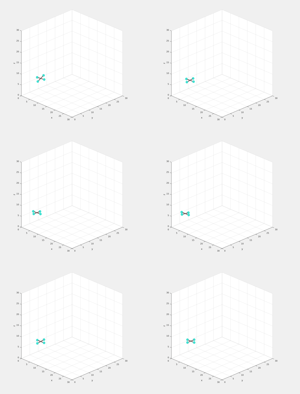
The result of NTCG on a quadrotor model is shown below. A random set of initial positions and velocities are given. The goal is to reach the same position with zero velocity. The solution is slightly sub-optimal as expected, but still satisfies all the torque constraints.
NCLDT
Non-Cooperative Locally Dynamic Trees
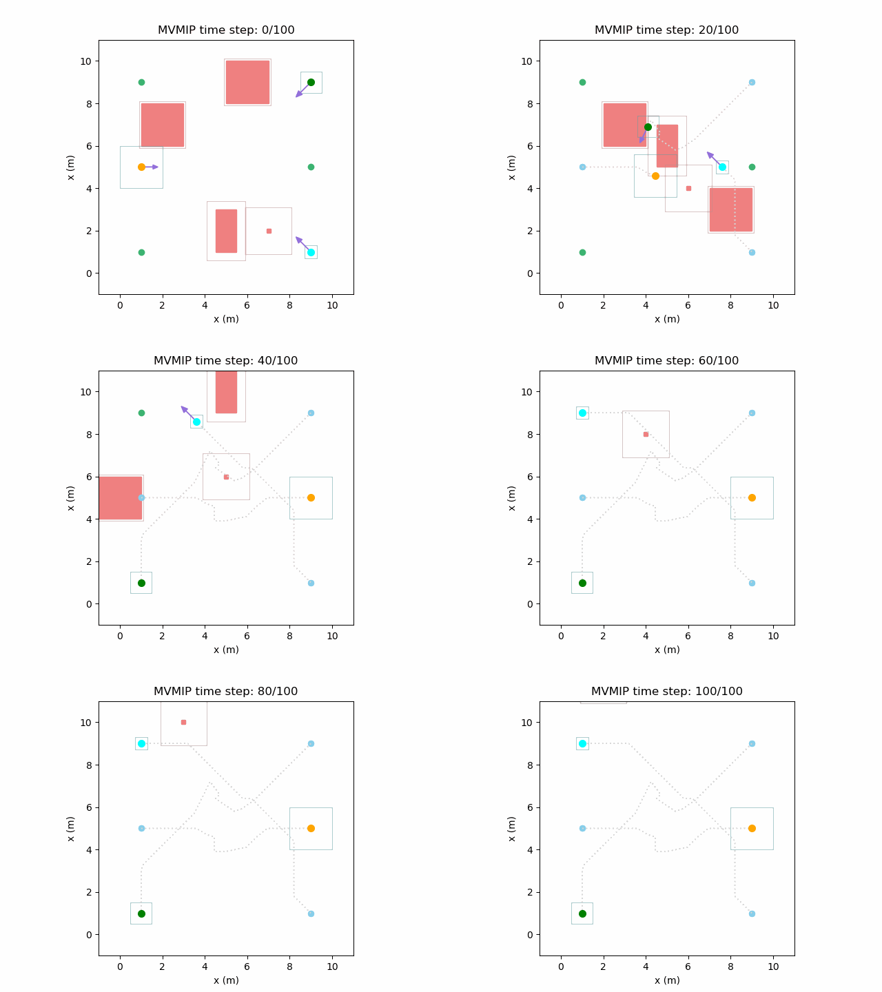
NCLDT is a novel probabilistic path planning algorithm that uses multiple dynamic trees to find obstacle-free paths in high dimensional and highly constrained spaces. It aims to be more efficient in finding solutions through narrow passages in state-space.
Unlike RRT’s, NCLDT grows (and decays) multiple trees. Each iteration samples and grows each active tree, while also looking at connection possiblities between the trees and the goal.
Single tree model
The randomness in NCLDT arises from the sampling of tree roots. The root of the tree is the only node that gets sampled in an unbiased manner. Once the root is sampled, the tree does not grow in all directions. Instead it can dynamically grow between two set directions. The first direction is towards the goal state. The second direction is perpendicular to the vector to the goal state, away from the initial state. The idea is that once a root has been sampled, the tree would have some idea on how to grow towards the goal. The two directio model enables the tree to actively grow around obstacles in its path, rather than rely on probabilistic guesses like RRT.
Depending on the proximity of obstacles in its path, each tree can grow in a direction between the two said directions. If there are no obstacles in the direction towards to goal, the tree is grown in this direction. If there are obstacles in this direction, the direction is changed to point more towards the perpendicular direction. If both the directions have obstacles close to the tree, the tree is is decayed.
While growing trees, a bunch of samples are made about some angular region in the direction of growth and the node closest to the farthest node in this direction is chosen and connected. This method ensures more consistent growth with lesser variance.
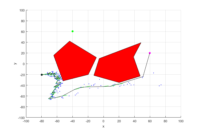
The dynamic growth of a single tree using the dual direction model is as shown. The results have been evaluated on a two dimensional environment. The red regions denote obstacles.
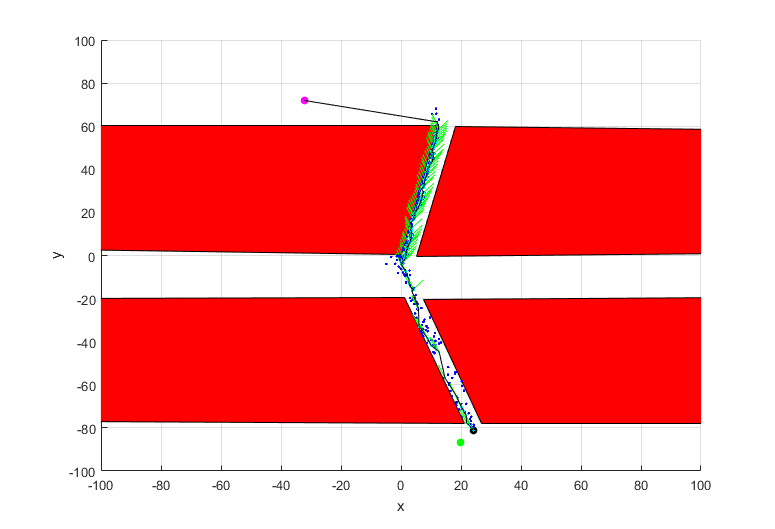
If a favorable root is sampled, a single tree is able to find its way through any narrow passage. This behavior is shown below.
Multi tree model
The goal of the algorithm is to have lots of these dynamic trees growing in the state space, enabling connections between trees. The inuition is that lots of root node samples would result in at least a few of the nodes being favorable. These roots would then grow trees around obstacles and through narrow passages. After these sub-paths are found, other trees would keep connecting with them till a path to the goal configuration is found.
The multi tree model introduces a few more complexities.
-
Root node sampling is very important: To help with this, initially, a bunch of samples are drawn radially from the initial state. They resemble samples on concentric hyper-spheres and are extended all the way to the goal configuration. The distance between the spheres can be chosen depending on the initial space complexity than can be afforded for the given state dimensions. The spherical sampling procedure gave the best empirical results out of the different techniques that were tried.
-
Trees that aren’t growing must be identified and decayed: This is done through a combination of tree growth and obstacle proximity. Each tree is given an energy level depending on its spread from its previous samples and the proximity of obstacles in the two primary directions. The total energy of the system is kept fixed and the energy of a decayed tree is set to zero. Each iteration, depending on the deficit in total energy, a number of tree nodes are sampled. This unified energy model helps in obtaining an elegant solution to the problem of decaying and spawning new trees, while also maintaining a balance between the two.
-
Joining different trees: Maintaining and joining trees to each other are also challenging due to the large number of samples in each tree. Instead of using a separate algorithmic approach to join trees, the dual direction model allows us to use the same approach. Instead of setting the first direction to the goal state, it can be set to the closest node of the tree to be connected to. The decision of whether to connect to the target or a nearby tree is made by using a probabilistic function that takes into account the number of trees that have connected to the goal as well as the proximity to other goal-connected trees. Once the trees have combined, they are treated as a single tree with their energies added.
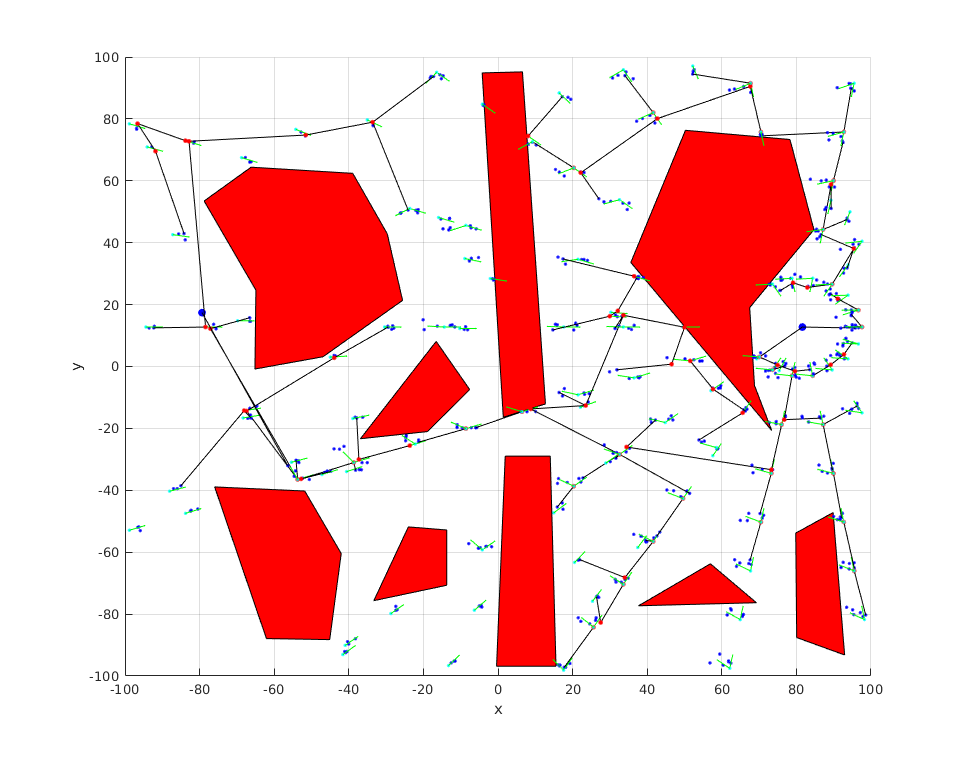
The result of the multi tree algorithm in a two dimensional setting is as shown.
ARDOP
Autonomous Robot Development Open-Source Platform
This one is one of my earliest robotics projects and what got me into the field!
ARDOP is a humanoid robot that was built to serve as an open-source platform for robotics. It was designed to be an economical way to learn and test algorithms for planning, control, perception and learning.
STL files for the parts are open-source and may be 3D printed. The robot consists of an upper body with two arms and a head. Each arm has five degrees of freedom and a gripper. The head has two degrees of freedom and houses a DUO 3D camera. Servo motors are used to actuate all the joints and are controlled using the PCA9685 PWM controller. The main processor used is the NVidia Jetson TK1, which interfaces with the motor controller and other hardware.
All the code is written in C++. Tests and simulations were run using MATLAB/Python, before being deployed on the hardware. The robot is able to identify objects and perform simple manipulation tasks as shown.
